In the Omniverse PoC post I said Isaac Sim issued only 2 draw calls for a 50-robot scene because geometry is resolved through “TLAS/BLAS traversed by vkCmdTraceRaysKHR.” That sentence does a lot of work and I never unpacked it.
This post unpacks it. No prior ray tracing knowledge assumed — if you know what a triangle and a 3D coordinate are, you have enough. At the end there is a complete runnable Python program that builds all of this from scratch and measures it, so none of the numbers here are hand-waved.
1. The only question ray tracing asks
Ray tracing is conceptually simple. To find the color of a pixel, you shoot a ray from the camera through that pixel and ask:
“What does this ray hit first?”
Everything else — shadows, reflections, global illumination — is that same question asked again from a different starting point. A reflection is just “shoot a new ray from where the last one landed.”
So the entire performance story of ray tracing is the cost of answering that one question.
2. Why the obvious answer is hopeless
The obvious answer: test the ray against every triangle, keep the closest hit.
Let’s price that out for a realistic frame:
1920 x 1080 pixels          ≈ 2,000,000 rays  (and that's just the primary rays)
a moderately detailed scene ≈ 5,000,000 triangles

2,000,000 x 5,000,000       = 10,000,000,000,000 ray-triangle tests per frame
Ten trillion. Per frame. At 60 FPS you would need six hundred trillion per second. An RTX 4090 is nowhere near that — it’s off by something like four orders of magnitude. And we haven’t added a single reflection or shadow ray yet.
Brute force isn’t slow. It’s impossible. So the entire field is built around not doing it.
3. The idea: boxes inside boxes
Here’s the trick, and it’s the same trick you already use without thinking about it.
Suppose I ask you to find one specific book in a large library. You don’t check every book. You do this:
Library
 └─ 3rd floor           ← "history is on 3, skip floors 1, 2, 4"
     └─ Aisle 12        ← skip the other 40 aisles
         └─ Shelf C     ← skip the other shelves
             └─ Book
Each step throws away almost everything. Five decisions instead of 100,000 checks.
Ray tracing does exactly this with boxes. You wrap groups of triangles in axis-aligned bounding boxes (AABBs — just “a box lined up with the X/Y/Z axes”), then wrap groups of boxes in bigger boxes, all the way up to one box containing the whole scene. That tree is called a BVH — Bounding Volume Hierarchy.
Does the ray miss the big box? Then it misses every triangle inside it. Discard millions of triangles with one test.
Does it hit? Descend into both children and repeat.
Reach a leaf? Now — and only now — do the expensive triangle test on the 4 triangles there.
The cost goes from O(N) to roughly O(log N). That’s the difference between 5,000,000 and about 20.
Why testing a box is cheap
This only pays off because a box test is much cheaper than a triangle test.
Ray vs. box is the “slab test”: for each of X, Y, Z, find where the ray enters and exits that pair of parallel planes. If the three intervals overlap, you hit. That’s a handful of subtractions, multiplications, and comparisons.
Ray vs. triangle is the Möller–Trumbore algorithm: two cross products, several dot products, a division, and three early-out branches — and then you also have to check whether the hit is closer than your current best.
So the strategy is: use the cheap test constantly to avoid the expensive test. You do more total tests, but the mix shifts overwhelmingly toward cheap ones. We’ll see this trade directly in the measurements.
4. So why two levels?
Everything above describes one BVH. But DXR and Vulkan RT deliberately split it into two:
BLAS (Bottom-Level Acceleration Structure) — a BVH over the actual triangles of one mesh, in that mesh’s own local coordinates.
TLAS (Top-Level Acceleration Structure) — a BVH over instances. Each instance is nothing but a pointer to a BLAS + a 3×4 transform matrix.
TLAS  (instances)
 ├─ Instance 0  : BLAS_ur16e     + transform(robot 0 is here, rotated this way)
 ├─ Instance 1  : BLAS_ur16e     + transform(robot 1)
 ├─ ...
 ├─ Instance 49 : BLAS_ur16e     + transform(robot 49)
 └─ Instance 50 : BLAS_warehouse + transform(the warehouse)

BLAS  (triangles, local space)
 ├─ BLAS_ur16e     : the UR16e mesh's triangle tree   ← built ONCE
 └─ BLAS_warehouse : the warehouse's triangle tree
The stamp analogy
Think of a rubber stamp.
BLAS is the stamp — you carve it once, carefully. It’s the shape itself.
TLAS is the list of where you pressed it on the paper — position and rotation, nothing more.
Fifty identical robots means you carve one stamp and record fifty press locations. You do not carve fifty stamps.
(If you prefer: a font works the same way. The letter A has one outline defined once; a page with 500 As stores 500 positions, not 500 outlines.)
This buys two specific things.
(a) Instancing is nearly free. Fifty robots cost one robot’s worth of geometry memory, plus fifty tiny transform matrices.
(b) Movement is cheap — and this is the important one. When a robot rotates a joint, its links are rigid bodies. The triangles themselves don’t deform; only the transform changes. So you rebuild the TLAS only — a tree over 50 items, which is trivial. The BLAS, a tree over millions of triangles, is never touched.
The exception: if geometry genuinely deforms — a skinned character, cloth, a soft body — you do have to refit or rebuild the BLAS, and that is expensive. You build it with ALLOW_UPDATE and refit rather than rebuild when you can. Rigid robot links are the friendly case; a bending cable is not.
Mapping it onto rasterization
If you come from a rasterizer background, here is the correspondence:
Rasterization
Ray tracing
Vertex / Index Buffer
BLAS
Walking the scene graph and issuing draws
TLAS
vkCmdDrawIndexed × N
vkCmdTraceRaysKHR × 1
In a rasterizer the CPU walks the scene every frame and submits a draw call per mesh section. In a ray tracer the whole scene already lives on the GPU as TLAS + BLAS; you issue one trace command and the RT cores walk the tree in hardware.
5. Let’s actually measure it
Talk is cheap. Here is a complete, dependency-free Python program that builds the same 50-robot scene three ways and counts the work:
Brute force — test every triangle
Single-level BVH — one big tree over all 25,000 world-space triangles
Two-level — TLAS over 50 instances + one shared BLAS
It asserts all three produce identical hits, then reports the cost.
"""
Two-level acceleration structure (TLAS / BLAS) demo.
Pure Python, no dependencies. Run: python bvh_demo.py
"""importmath,randomrandom.seed(7)# ---------------------------------------------------------------- counters
classCounter:def__init__(self):self.tri=0;self.box=0defreset(self):self.tri=0;self.box=0C=Counter()# ---------------------------------------------------------------- vec3
defsub(a,b):return(a[0]-b[0],a[1]-b[1],a[2]-b[2])defadd(a,b):return(a[0]+b[0],a[1]+b[1],a[2]+b[2])defcross(a,b):return(a[1]*b[2]-a[2]*b[1],a[2]*b[0]-a[0]*b[2],a[0]*b[1]-a[1]*b[0])defdot(a,b):returna[0]*b[0]+a[1]*b[1]+a[2]*b[2]defnorm(a):l=math.sqrt(dot(a,a));return(a[0]/l,a[1]/l,a[2]/l)# ---------------------------------------------------------------- ray tests
defray_tri(orig,dirv,tri):"""Moller-Trumbore. The EXPENSIVE test."""C.tri+=1v0,v1,v2=trie1=sub(v1,v0);e2=sub(v2,v0)p=cross(dirv,e2);det=dot(e1,p)ifabs(det)<1e-9:returnNoneinv=1.0/dettvec=sub(orig,v0)u=dot(tvec,p)*invifu<0oru>1:returnNoneq=cross(tvec,e1)v=dot(dirv,q)*invifv<0oru+v>1:returnNonet=dot(e2,q)*invreturntift>1e-6elseNonedefray_box(orig,dirv,bmin,bmax,tmax):"""Slab test. The CHEAP test."""C.box+=1t0,t1=1e-6,tmaxforiinrange(3):ifabs(dirv[i])<1e-12:iforig[i]<bmin[i]ororig[i]>bmax[i]:returnFalsecontinueinv=1.0/dirv[i]a=(bmin[i]-orig[i])*invb=(bmax[i]-orig[i])*invifa>b:a,b=b,aifa>t0:t0=aifb<t1:t1=bift0>t1:returnFalsereturnTrue# ---------------------------------------------------------------- BVH build
deftri_bounds(tri):xs=[v[0]forvintri];ys=[v[1]forvintri];zs=[v[2]forvintri]return(min(xs),min(ys),min(zs)),(max(xs),max(ys),max(zs))defmerge(b1,b2):(a0,a1,a2),(a3,a4,a5)=b1(c0,c1,c2),(c3,c4,c5)=b2return(min(a0,c0),min(a1,c1),min(a2,c2)),(max(a3,c3),max(a4,c4),max(a5,c5))classNode:__slots__=("bmin","bmax","left","right","items")def__init__(self):self.left=self.right=None;self.items=Nonedefbuild_bvh(items,bounds_of,leaf_size=4):"""Median-split BVH. bounds_of(item) -> (bmin, bmax)"""node=Node()b=bounds_of(items[0])foritinitems[1:]:b=merge(b,bounds_of(it))node.bmin,node.bmax=biflen(items)<=leaf_size:node.items=items;returnnodeext=[node.bmax[i]-node.bmin[i]foriinrange(3)]axis=ext.index(max(ext))# split the longest axis
items=sorted(items,key=lambdait:(bounds_of(it)[0][axis]+bounds_of(it)[1][axis]))mid=len(items)//2node.left=build_bvh(items[:mid],bounds_of,leaf_size)node.right=build_bvh(items[mid:],bounds_of,leaf_size)returnnodedefcount_nodes(n):return1ifn.itemsisnotNoneelse1+count_nodes(n.left)+count_nodes(n.right)defbvh_depth(n):return1ifn.itemsisnotNoneelse1+max(bvh_depth(n.left),bvh_depth(n.right))# ---------------------------------------------------------------- traversal
deftrace_bvh_tris(node,orig,dirv,best):"""BVH whose leaves hold triangles."""ifnotray_box(orig,dirv,node.bmin,node.bmax,best):returnbestifnode.itemsisnotNone:fortriinnode.items:t=ray_tri(orig,dirv,tri)iftisnotNoneandt<best:best=treturnbestbest=trace_bvh_tris(node.left,orig,dirv,best)best=trace_bvh_tris(node.right,orig,dirv,best)returnbestdeftrace_tlas(node,orig,dirv,best):"""TLAS: leaves hold instances -> move ray to object space, descend into BLAS."""ifnotray_box(orig,dirv,node.bmin,node.bmax,best):returnbestifnode.itemsisnotNone:forinstinnode.items:# world -> object space. Translation only here, so a subtract suffices.
# With rotation you would apply the inverse 3x4 matrix to orig AND dir.
lo=sub(orig,inst.offset)best=trace_bvh_tris(inst.blas,lo,dirv,best)returnbestbest=trace_tlas(node.left,orig,dirv,best)best=trace_tlas(node.right,orig,dirv,best)returnbest# ---------------------------------------------------------------- scene
classInstance:__slots__=("blas","offset","bmin","bmax")defmake_robot_mesh(n_tris):"""A blob of triangles inside the local box [-0.5, 0.5]^3."""tris=[]for_inrange(n_tris):cx=random.uniform(-0.4,0.4);cy=random.uniform(-0.4,0.4);cz=random.uniform(-0.4,0.4)defv():return(cx+random.uniform(-0.08,0.08),cy+random.uniform(-0.08,0.08),cz+random.uniform(-0.08,0.08))tris.append((v(),v(),v()))returntrisTRIS_PER_ROBOT,N_ROBOTS,N_RAYS=500,50,200robot=make_robot_mesh(TRIS_PER_ROBOT)offsets=[(i*1.6-7.2,0.0,j*1.6-3.2)foriinrange(10)forjinrange(5)][:N_ROBOTS]# world-space triangle soup (brute force + single-level BVH)
world_tris=[tuple(add(v,off)forvintri)foroffinoffsetsfortriinrobot]# two-level: ONE blas, N instances
blas=build_bvh(robot,tri_bounds)instances=[]foroffinoffsets:inst=Instance()inst.blas=blas# shared! built once
inst.offset=offinst.bmin=add(blas.bmin,off)inst.bmax=add(blas.bmax,off)instances.append(inst)tlas=build_bvh(instances,lambdai:(i.bmin,i.bmax),leaf_size=2)# single-level BVH over every world triangle
flat_bvh=build_bvh(world_tris,tri_bounds)# ---------------------------------------------------------------- rays
eye=(0.0,6.0,-14.0)rays=[(eye,norm(sub((random.uniform(-8,8),random.uniform(-1,1),random.uniform(-4,4)),eye)))for_inrange(N_RAYS)]defrun(fn):C.reset()return[fn(o,d)foro,dinrays],C.tri,C.boxdefbrute(orig,dirv):best=float("inf")fortriinworld_tris:t=ray_tri(orig,dirv,tri)iftisnotNoneandt<best:best=treturnbesth_brute,tri_b,box_b=run(brute)h_flat,tri_f,box_f=run(lambdao,d:trace_bvh_tris(flat_bvh,o,d,float("inf")))h_two,tri_t,box_t=run(lambdao,d:trace_tlas(tlas,o,d,float("inf")))defsame(a,b):returnall(abs(x-y)<1e-6or(x==float("inf")andy==float("inf"))forx,yinzip(a,b))print(f"scene: {N_ROBOTS} instances x {TRIS_PER_ROBOT} tris = {len(world_tris):,} triangles")print(f"correctness: flat==brute {same(h_flat,h_brute)} two-level==brute {same(h_two,h_brute)}")print(f"{'method':<22}{'triangle tests':>18}{'AABB tests':>14}{'tri/ray':>10}")print(f"{'brute force':<22}{tri_b:>18,}{box_b:>14,}{tri_b/N_RAYS:>10.1f}")print(f"{'single-level BVH':<22}{tri_f:>18,}{box_f:>14,}{tri_f/N_RAYS:>10.1f}")print(f"{'two-level TLAS+BLAS':<22}{tri_t:>18,}{box_t:>14,}{tri_t/N_RAYS:>10.1f}")print(f"speedup vs brute: single-level {tri_b/tri_f:.1f}x two-level {tri_b/tri_t:.1f}x")print(f"single-level BVH : {count_nodes(flat_bvh):,} nodes, depth {bvh_depth(flat_bvh)}")print(f"two-level : {count_nodes(blas):,} BLAS nodes + {count_nodes(tlas):,} TLAS nodes")
Results
scene: 50 instances x 500 tris = 25,000 triangles
rays : 200
correctness: flat==brute True   two-level==brute True
rays that hit something: 85/200

method                    triangle tests    AABB tests   tri/ray
------------------------------------------------------------------
brute force                    5,000,000             0   25000.0
single-level BVH                   3,494        14,512      17.5
two-level TLAS+BLAS                3,150         9,475      15.8
------------------------------------------------------------------
speedup vs brute: single-level 1431.0x   two-level 1587.3x

memory / build:
  brute force        : 25,000 tris stored, no tree
  single-level BVH   : 25,000 tris stored, 16,383 nodes, depth 14
  two-level          : 500 tris stored (shared BLAS), 255 BLAS + 63 TLAS nodes
  -> geometry memory : 50x less for the two-level build

cost of moving all 50 robots one frame:
  single-level BVH   : rebuild over 25,000 triangles
  two-level          : rebuild TLAS over 50 instances  (BLAS untouched)
  -> rebuild input   : 500x smaller
6. Reading those numbers honestly
The hierarchy is the whole game. 25,000 triangle tests per ray → 17.5. A 1,431× reduction, and the tree is only 14 levels deep. That is the O(N) → O(log N) claim, measured.
The trade is real and visible. The BVH does 14,512 AABB tests to avoid 5 million triangle tests. It performs more tests overall — it just made almost all of them cheap ones. That’s the bargain, in numbers.
Now the part people get wrong. Look again at single-level vs two-level:
Two levels barely helps traversal speed. Roughly a wash. If you assumed TLAS/BLAS exists to make tracing faster, the data says otherwise.
The actual reasons are the last two blocks of output:
50× less geometry memory. One BLAS, not fifty copies. On a real scene this is the difference between fitting in VRAM and not.
500× smaller rebuild. Move all 50 robots and you rebuild a tree over 50 instances instead of 25,000 triangles. Every frame. This is why animated scenes are viable at all.
So the honest one-line summary: two levels exist for memory and for dynamic updates, not for raw traversal throughput. That distinction matters when you’re deciding whether to merge meshes into one BLAS (fewer instances, faster traversal, but now they can’t move independently) or split them (more instances, cheaper updates).
Where this toy differs from real hardware
I want to be clear about what the demo does not model, so nobody over-reads it:
Translation only, no rotation. Real instances carry a full 3×4 matrix, and you must transform the ray direction too, not just the origin.
Median split, not SAH. Production builders use the Surface Area Heuristic, which produces meaningfully better trees.
Test counts, not time. On an RTX GPU, box and triangle tests run on fixed-function RT cores, so the cost ratio between them is nothing like it is in Python. The counts show the algorithmic win; they do not predict milliseconds.
One ray at a time. Real GPUs trace 32 rays per warp in lockstep — which brings us to the last section.
7. Back to the PoC: why this explained the profiler
Two findings from the Omniverse post come straight out of the structure above.
Why Isaac Sim showed 2 draw calls
Because the scene is not rasterized. It lives on the GPU as TLAS + BLAS and is traversed by vkCmdTraceRaysKHR. Instanced geometry never passes through vkCmdDrawIndexed at all. The 2 draw calls that appeared were the ImGui overlay.
So “2 draw calls” doesn’t mean efficient — it means that code path isn’t being used. Comparing it against Unreal’s 10,733 is comparing a number to the absence of that number.
Why RTCORE throughput was only 5.3% while VRAM hit 34%
This is the part the toy demo can’t show you, and it’s the most practically useful.
BVH traversal is branchy and memory-incoherent. A GPU executes 32 threads per warp in lockstep. For primary camera rays that’s fine — neighbouring pixels shoot nearly parallel rays that walk nearly the same path down the tree.
Reflection rays destroy that. They scatter in 32 different directions and descend 32 different branches. Every thread wants a different node from memory, so cache lines thrash and the warp stalls waiting on all of them.
Meanwhile the actual ray-triangle intersection is fixed-function silicon and finishes almost instantly — hence RT cores idle at 5.3% while VRAM throughput sits at 34%.
The bottleneck in ray tracing is usually pointer chasing, not intersection math.
That reframes optimization completely. Adding RT cores wouldn’t have helped that frame. Reducing reflection rays, tightening the roughness cutoff, or improving BVH quality to shorten traversal — those would.
Why 50 robots barely changed Isaac Sim’s render cost
Recall the measurement: RTX rendering went 13.52 ms → 10.76 ms when 50 robots were added.
Now it should be unsurprising. Adding instances reuses the same BLAS and grows the TLAS by 50 entries, deepening the tree only logarithmically. Ray tracing cost tracks pixels and ray depth, not triangle count.
Compare Unreal in the same scenario: 10,733 draw calls and 2.14 ms rebuilding Lumen’s distance field, both scaling with the amount of moving geometry. Two fundamentally different cost curves — which was the real conclusion of that PoC, and the reason a single FPS comparison couldn’t capture it.
One honest caveat, same as in the original post: I did not verify from the capture that Isaac Sim actually shares a single BLAS across those 50 robots (it would if they’re USD instanced prims). But BLAS construction is a one-time cost either way, so the scaling conclusion holds regardless.
8. The real API
If you want to build this for real, the names to search for:
Rule of thumb that follows directly from §6: BLAS for static meshes → PREFER_FAST_TRACE. TLAS rebuilt every frame → PREFER_FAST_BUILD. You’re building the TLAS constantly and tracing through it briefly; you build the BLAS once and trace through it forever.
Summary
Ray tracing asks one question — what does this ray hit first? — and brute force is off by orders of magnitude.
A BVH wraps geometry in nested boxes so one cheap box test discards millions of triangles. Measured: 25,000 → 17.5 triangle tests per ray.
BLAS = the stamp (triangles, local space, built once). TLAS = where you pressed it (instances = BLAS pointer + transform).
Two levels exist for memory (50×) and update cost (500×) — not for traversal speed, which was within 10%.
On real hardware the bottleneck is incoherent memory access during traversal, not intersection math. That’s why RT cores sat at 5.3% while VRAM was at 34%.
Consequently, RT cost scales with pixels and ray depth, while rasterization scales with draw calls and moving geometry. Different curves — which is exactly why “which engine is faster” was the wrong question.
We had a concrete decision to make: for a warehouse-scale robotics digital twin, do we build on Isaac Sim (Omniverse Kit) or stay on Unreal Engine, which the team already knows?
The naive way to answer this is to run both, look at the FPS counter, and pick the faster one. That answer would have been “Unreal, by a mile” — and it would have been wrong, or at least wrong for the reasons people would have assumed. So instead of trusting the frame counter, I captured both runtimes under NVIDIA Nsight Graphics and read the GPU counters.
This post is the write-up of that PoC: what the platform actually is, what the profiler actually showed, and — most importantly — which of those numbers are comparable across two different renderers and which are not. The second part matters more than the first.
1. What Omniverse actually is
Before benchmarking it helps to be precise about what is being benchmarked. “Omniverse” is not an engine. It is a microservice runtime (Omniverse Kit) on which applications are composed from extensions.
The relevant architectural properties:
Extension-based composition. Everything — the viewport, the physics scene, the ROS bridge — is an extension loaded into the Kit runtime. There is no monolithic editor binary the way there is in Unreal.
Kit micro services + service facilities. DB, work queue, metrics, and logging are first-class service facilities. This is what makes headless/fleet deployment (multi-server, cloud) a configuration change rather than a port.
USD as the scene contract. The stage is OpenUSD, not a proprietary asset database. Interop with Maya/Blender/Unreal goes through USD via Omniverse Connect rather than through import/export.
The pieces that mattered for us
Layer
Component
Why we cared
Core
Kit
The runtime everything else is an extension of
Core
Connect
USD LiveLink into Unreal / Maya / Blender
Core
Nucleus
Cloud-native asset DB + versioning; feeds Omniverse Farm
First gap found: neither Kit nor Isaac Sim ships a runtime monitoring extension. There is no built-in equivalent of stat unit / stat gpu that streams structured per-subsystem timings out of the process. Everything below had to be captured externally with Nsight. For a production digital twin this is a real gap — you cannot alert on what you cannot export.
2. Test setup
Both runtimes on the same box, same monitor, same scene asset.
Scenario A — the warehouse scene with an action sequence playing.
Scenario B — 50 × UR16e, all executing a RotateZ action simultaneously.
Counters collected: GPU utilization, frame time, SM throughput, VRAM throughput, L2 throughput + sector hit-rate, draw calls, dispatches, SM warp occupancy.
Establishing environment parity (and failing to, honestly)
This was the hardest part of the PoC and it is worth being explicit about, because it bounds every conclusion below.
Problem: material loss on export. Getting the same stage into Unreal meant going Isaac Sim → FBX/glTF → Unreal, and material information does not survive that trip. Blender as an intermediate shows what actually crosses the boundary — geometry, and not much else:
Mitigation. Rather than fight it, we levelled down to the lowest common denominator:
Stripped materials in Isaac Sim so both sides render untextured geometry.
Standardised lighting on Rect Lights.
Disabled post-processing in Unreal via Show Flags — Bloom, Color Grading, DoF, Eye Adaptation, Motion Blur, Tonemapper, Vignette all off.
Resulting baselines:
Unreal Engine
Isaac Sim
Caveat I want on the record: the captures were ultimately taken with Point Light in Unreal and Rect Light in Isaac Sim. That is not a cosmetic difference. A point light is an analytic delta-distribution light; a rect light is an area light that has to be sampled. Under a ray-traced integrator that changes the shading cost per pixel directly. So the numbers below are a comparison of two configured pipelines, not of two engines under identical optical conditions. Read them as “what each stack does when set up the way its own defaults push you,” not as a controlled A/B.
3. How to read these counters
One diagram is worth keeping in mind for the whole results section, because every number below is a statement about one level of this hierarchy:
SM Throughput — how hard the shader cores are working. Instructions issued vs. peak issue rate.
SM Warp Occupancy — how many of the SM’s warp slots hold a resident warp. (Active Warps / Theoretical Max Warps) × 100. On Ada the theoretical max is 48 warps/SM. Nsight reports “Unallocated Warps in Active SMs” as a separate row — that row is empty slots, not work.
L2 Throughput / Sector Hit-Rate — how much traffic the last-level cache is absorbing. High throughput with a high hit-rate means the working set fits and is being hammered; a hit-rate drop means you fell through to DRAM.
VRAM Throughput — DRAM bandwidth, split read/write. The read/write ratio is a fingerprint of the workload.
The interpretive rule I applied throughout: if SM throughput is low while VRAM/L2 throughput is high, the frame is latency- or bandwidth-bound, not math-bound. Low on both means the GPU is waiting on someone else — usually the CPU.
4. Scenario A — warehouse scene with action sequence
Unreal Engine
Isaac Sim
Light setup
Point Light
Rect Light
FPS (before play)
92.80 – 107.21
76.91 – 116.50
FPS (play & run)
75.59 – 104.21
48.34 – 60.15
Avg FPS
100.01 → 89.90
96.71 → 54.25
Frame time (capture)
8.29 ms
14.12 ms
API
D3D12
Vulkan
GPU contexts
1 × D3D12 (8.86 ms)
3 × VkContext (8.29 + 1.07 + 3.65 ms)
Dispatches
2 + 7 + 2 = 11
22 compute + 7 ray tracing + 15 OptiX/CUDA
Draw calls (vkCmdDrawIndexed / equiv.)
8 + 2 + 8 + 1 = 19
2 (UI only)
SM throughput
6.4 %
12.9 %
VRAM throughput
8.8 % (R 5.5 / W 3.2)
34.0 % (R 10.5 / W 23.5)
L2 throughput
9.9 % (hit-rate 82.6 %)
32.4 % (hit-rate 90.1 %)
Occupancy — unallocated
6.8 warps / 14.2 %
29.0 warps / 60.5 %
Occupancy — compute
4.0 warps / 8.3 %
11.2 warps / 23.4 %
Occupancy — pixel
0.6 warps / 1.3 %
0.3 warps / 0.7 %
Occupancy — vtx/tess/geom
0.1 warps / 0.2 %
0.0 warps / 0.0 %
Unreal capture
A textbook deferred frame. Scene occupies 5.87 ms of the 8.29 ms frame, and inside it the marker track reads DistanceFieldA… → BasePass (0.89 ms) → FVirtualShadowMapArray::BuildPageAllocation → DiffuseIndirect → LumenScreen… → PostProcessing → TSR. Note what that spells out: Lumen and Virtual Shadow Maps are on. Unreal here is not doing “plain rasterization” — it is running its own software-traced GI. The async compute queue is live in parallel.
Isaac Sim capture
Structurally different. Three Vulkan contexts with batched submission:
Geometry / direct — G-buffer, sampled direct lighting, reflections
Indirect diffuse — global illumination
Post — translucency, anti-aliasing (DLSS SR / TAA)
The marker track is the interesting part. RTX Rendering is 13.52 ms of the 14.12 ms frame, RTX Render Tile is 11.97 ms of that, and inside it:
Reflections — 4.50 ms
Reflections RT Sampled — 4.25 ms
then Indirect Diffuse, Translucency, AntiAliasing, DLSS RenderOp, DLSS Evaluation
Ray-traced reflections alone are ~33 % of the frame. That is the single largest line item, and it is a quality setting, not a structural property of Isaac Sim. Actions: raise the roughness cutoff so glossy surfaces fall back to a cheaper probe, reduce reflection sample count, or cap reflection bounce depth. The warehouse floor in that scene is a mirror — visible in the viewport screenshot — and mirrors are exactly what makes RT reflections expensive.
Also worth noting: vkCmdTraceRaysKHR (4) shows at 4.25 ms, and RTCORE throughput is only 5.3 %. The RT cores are not saturated. The cost is not in triangle-ray intersection; it is in the incoherent memory access that BVH traversal and reflection-ray shading generate. Which the VRAM counter confirms — 34 % throughput, and write-dominant (23.5 % write vs 10.5 % read), the signature of a denoise/accumulate pipeline writing out radiance and history buffers every frame.
5. Scenario B — 50 robots
Unreal Engine
Isaac Sim
Robots
50 × UR16e, RotateZ
50 × UR16e, RotateZ
FPS (play & run)
93.89 – 104.54
42.15 – 49.42 (66.67 when few robots in frustum)
Frame time
7.67 ms
15.45 ms
GPU contexts
2
4
Dispatches
96
24 compute + 7 ray tracing + 15 OptiX/CUDA
Draw calls
10,733 (incl. UI)
2 (UI only)
SM throughput
11.9 %
11.9 %
VRAM throughput
11.5 % (R 3.6 / W 7.8)
26.9 % (R 7.6 / W 19.2)
L2 throughput
20.6 % (hit-rate 95.5 %)
27.2 % (hit-rate 91.9 %)
Occupancy — unallocated
36.9 warps / 76.9 %
22.6 warps / 47.1 %
Occupancy — pixel
5.9 warps / 12.2 %
0.0 warps / 0.1 %
Occupancy — vertex
3.5 warps / 7.3 %
0.0 warps / 0.0 %
Occupancy — compute
0.0 warps / 0.0 %
1.8 warps / 3.7 %
Occupancy — unattributed
0.0 warps / 0.0 %
5.4 warps / 11.2 %
Three things in this table are not what they look like
(a) 10,733 vs 2 draw calls is not an efficiency result.
This is the number most likely to be quoted out of context, so: Isaac Sim issues 2 draw calls because the scene is not rasterized at all. Geometry is resolved through ray-tracing acceleration structures — TLAS/BLAS built once, then traversed by vkCmdTraceRaysKHR. Instanced geometry never passes through vkCmdDrawIndexed. The 2 draw calls that do appear are the ImGui overlay.
Draw-call count is therefore not a comparable metric across these two renderers. It measures a submission model that only one of them uses. Comparing them is a category error.
(b) 10,733 draw calls in Unreal is a config problem, not an engine property.
50 robots → ~215 draw calls per robot. A UR16e has 6–7 links. That means the imported meshes are being submitted per-section with no instancing and no Nanite, which is exactly what you get from a raw FBX import chain that also lost its materials. The occupancy row corroborates it: 76.9 % of warp slots unallocated with pixel warps at 12.2 % and vertex at 7.3 % — SMs are active almost the whole frame but mostly empty, the classic signature of many small draws with poor warp packing. Enable instancing or Nanite on those meshes and this number should collapse.
(c) Unreal got faster with 50 more robots (8.29 → 7.67 ms). Treat that as a methodology flag, not a finding.
An engine does not speed up when you give it 500× the draw calls. The likely explanation is that the two captures do not share a camera pose or view frustum — and the Scenario A capture, at 8.29 ms with SM throughput at 6.4 % and everything else in single digits, looks like a frame where the GPU was largely idle waiting on present or CPU submission. The Scenario B capture shows the GPU genuinely busy (SM 11.9 %, L2 20.6 % at a 95.5 % hit-rate). Different bottlenecks, so the two frame times are not on the same scale. Fixing this needs a locked camera and a fixed-path flythrough on both sides.
What actually costs time in each frame
Unreal, 50 robots (7.67 ms frame, 5.75 ms active):
UpdateGlobalDistanceField — 2.14 ms, with Clipmap: 0 / Clipmap: 1 CacheType:Movable (1.58 ms) and BuildPageUpdateTiles 600 (1.43 ms)
Scene — 3.39 ms on the 3D queue, plus 4.53 ms on the async compute queue (AccessModePass[AsyncCompute], LumenSceneLighting, DiffuseIndirectAndAO 1.17 ms)
That first line is the real story on the Unreal side: 28 % of the frame is rebuilding Lumen’s global signed distance field, because 50 articulated robots marked Movable dirty the SDF clipmaps every single frame. This is a cost that scales with moving geometry, not with geometry. If we did not need Lumen GI for this workload — and for a robotics twin we largely do not — turning it off recovers roughly a third of the frame outright.
Isaac Sim, 50 robots (15.45 ms frame, 11.84 ms active):
Reflections — 3.27 ms, Reflections RT Sampled — ~3.0 ms
then Indirect, AntiAliasing, DLSS Render / DLSS Evaluation
Compare against Scenario A: RTX rendering went 13.52 ms → 10.76 ms while the scene gained 50 articulated robots. Isaac Sim’s render cost is essentially independent of robot count here. It is dominated by a fixed per-pixel ray-tracing budget — reflections above all — not by scene complexity. That is the expected scaling behaviour of a ray tracer: cost tracks pixels and ray depth, and geometry only shows up as BVH-traversal depth.
6. The finding the render captures do not explain
Look back at Scenario A:
Isaac Sim   Before Play: 96.71 avg FPS   →   Play & Run: 54.25 avg FPS
Unreal      Before Play: 100.01 avg FPS  →   Play & Run:  89.90 avg FPS
Isaac Sim loses 44 % of its frame rate the moment simulation starts — while, as shown above, GPU render cost barely moves. That delta is not in any of these Nsight captures, because Nsight captured the graphics queue.
The cost is on the other side of the frame: PhysX 5.0 articulation stepping, and USD stage update / Fabric synchronisation. Every simulated joint produces transform writes that must propagate through the stage before the renderer can consume them, and Kit’s update loop is where that happens.
This is the concrete consequence of the monitoring gap noted in §1 — we found the largest single performance effect in the entire PoC and could not attribute it, because there is no CPU-side instrumentation exported from the Kit runtime. It is the top item on the follow-up list for a reason.
The headline is easy to state and easy to misread: Unreal renders this scene about 2× faster. The correct reading is that the two runtimes are bound by different things, both are running well under 20 % SM throughput on a 4090, and neither frame time is anywhere near a hardware limit. This is a configuration difference far more than a capability difference.
8. Recommendation
Isaac Sim where the simulation is the product:
Robotics simulation and controller testing (PhysX 5.0 articulations)
Synthetic data generation for perception training (Replicator, segmentation GT, domain randomization)
Interactive applications with a hard >60 FPS budget
Teams already invested in the Unreal ecosystem
What we are actually proposing: not a choice — a split. Isaac Sim as the physics and sensor authority, Unreal as a visualization client, coupled over USD via Omniverse Connect. Each side then runs in the regime it is good at, and the 2× render gap stops being a decision input, because Isaac Sim runs headless with rendering disabled for the RL/data-generation workloads where throughput actually matters.
Before committing, the cheap wins are worth taking on both sides:
Isaac Sim — cap RT reflection roughness cutoff and sample count. That is a ~30 % frame-time line item under direct control.
Unreal — disable Lumen for the twin workload (recovers the 2.14 ms SDF rebuild), and enable instancing/Nanite on the imported robot meshes to kill the 10,733 draw calls.
9. Open items
Ranked by how much they would change the conclusions:
CPU / memory profiling instrumentation. The 96 → 54 FPS drop at simulation start (§6) is the largest unexplained effect in the PoC and it is entirely CPU-side. Nsight Systems trace of the Kit update loop, isolating PhysX stepping from USD/Fabric sync.
Re-run with locked camera and matched lighting. The Scenario A/B inconsistency (§5c) and the Point-vs-Rect light mismatch (§2) both cap how far these numbers can be pushed. Fixed-path flythrough, identical light type, on both sides.
Build a monitoring extension for Kit. No structured per-subsystem timing export exists. For production this is a blocker, and Kit’s service-facility model (metrics is already a first-class facility) is the right place to hang it.
Initialization latency. Time from Play to first stepped simulation frame — untouched so far, and it dominates iteration speed in practice.
Sequence storage footprint. Bytes-per-frame for recorded sequences, which determines whether long-horizon captures are viable at all.
Scaling curve, not points. Sweep robot count (1 / 10 / 50 / 200) and sensor configuration. Two data points cannot distinguish linear from constant scaling — and §5 suggests Isaac Sim’s render cost may be close to constant, which would be the strongest argument in its favour.
Closing note
The one lesson I would carry out of this PoC: frame rate is a scalar summary of a vector quantity. Isaac Sim “lost” by 2× on FPS while being bound by ray-traced reflection cost that is a slider, and Unreal “won” while spending 28 % of its frame rebuilding a distance field for GI we do not need. Neither of those facts is visible from the frame counter, and both change the decision.
In the previous post, we looked at the history of Gaussian Splatting. Now, let’s look at some experiments with 3D Gaussian Splatting and validation of the results. Also, I want to learn this as kinda of like top-down approach. So, I will start with running the 3DGS pipeline on a custom dataset and then analyze the results. The goal is to understand how the pipeline works end-to-end and to validate that it produces reasonable results on a real-world scene.
Objective
It was to run the 3DGS implementation en-to-end on a custom dataset. (self-capmtured indoor scene) for the first time and validate the results.
Experience the full pipeline: COLMAP SfM → 3DGS training → point cloud output → viewer visualization
Verify that training converges and produces visually reasonable results on a custom scene
The meta for first time running the 3DGS pipeline on playroom dataset. (225 Images). My GPU was NVIDIA GeFORCE RTX 2070 Super (8GB VRAM) and the training took about 2 days to complete. The viewer were used to visualize the output point cloud.
The config was as follows:
Namespace(data_device='cuda',
eval=False, # ← BUG: no train/test split → metrics are NaNimages='images',
resolution=-1, # original resolutionsh_degree=3, # Spherical Harmonics degreesource_path='C:\\Users\\skcjf\\project\\gaussian-splatting\\data\\my_scene\\playroom',
model_path='./output/858ba1ea-e',
train_test_exp=False,
white_background=False
)
Results
Training time: ~2 days (RTX 2070 Super)
Iterations: 30,000 (checkpoints at 7,000 and 30,000)
Then I did not get the results that I expected because I did not add –eval flag to the config, so I got NaN for all the metrics. But the point cloud output looked reasonable and the viewer visualization showed a decent reconstruction of the scene. The PSNR, SSIM, and LPIPS metrics were not computed due to the missing evaluation flag, so I will need to rerun with –eval to get those quantitative results.
Iteration Comparison in Point Cloud Output:
Iteration
7K
30K
Front-facing view (looking into the room): 7k and 30k are nearly identical
Looking up at the ceiling: visible holes/gaps → likely insufficient training views from upward angles, or densification did not cover that region adequately
Problem Encountered:
Output folder names are random hashes (e.g. 858ba1ea-e), so locating the actual results was initially confusing
No build errors; used a separate Python virtual environment
Training took ~2 days on RTX 2070 Super, which saturated the GPU entirely (couldn’t even run YouTube simultaneously)
4 total attempts, 3 failed/aborted before the successful run
Second Run with Evaluation
Objective
Run 3DGS on a standard benchmark dataset with --eval enabled to obtain real quantitative metrics (PSNR/SSIM/LPIPS) for the first time. This fixes the [[3DGS First Run]] problem where eval=False produced NaN metrics.
Validate that the 3DGS pipeline produces results consistent with the original paper
Establish a quantitative baseline for future experiments (hyperparameter tuning, ablation)
Learn the full evaluation pipeline: train → render → metrics
I choose to use Google Colab for this run to leverage a more powerful GPU (A100 40GB with High RAN) and faster training times. Then, I ran multiple data (tandt_db / Mip-NeRF 360 dataset) as well to validate the results from paper.
The config was as follows:
Namespace(sh_degree=3,
source_path='/content/gaussian-splatting/data/tandt/train',
model_path='/content/drive/MyDrive/3dgs_output/train', # NOTE: mislabeled — actual scene is "train"images='images',
resolution=-1, # original resolutionwhite_background=False,
train_test_exp=False,
data_device='cuda',
eval=True # FIXED from First Run — train/test split enabled)
Results
Metric
Value
PSNR
22.12
SSIM
0.822
LPIPS
0.196
Gaussians
1,095,714
Iterations
30,000 (checkpoints at 7,000 / 30,000)
GPU
A100 40GB (Google Colab)
These were the metrics using for the dataset: tandt_db(train). The PSNR and SSIM values are consistent with the original 3DGS paper, which reported PSNR around 22-23 and SSIM around 0.8 for similar scenes. The LPIPS value of 0.196 also indicates a reasonably good perceptual quality compared to the ground truth images. The number of Gaussians (1,095,714) is also in line with expectations for a scene of this complexity.
Problems Encountered
Mip-NeRF 360 dataset URL (storage.googleapis.com) returned 404 — dead link
Initial !unzip extracted to wrong path → Could not recognize scene type! error. Fixed by ensuring sparse/0/ was in the correct location.
What I Learned
--eval is mandatory for quantitative evaluation — without it, no train/test split occurs
3DGS with default config on standard benchmarks reproduces paper results — the pipeline works
A100 vs RTX 2070 Super is a massive speed difference — Colab is the practical choice for experimentation
Dataset URL availability is not guaranteed — always have backup sources
Third Run with Mip-NeRF 360 Dataset
Objective
Experimentally verify the impact of 3 key 3DGS hyperparameters on the Mip-NeRF 360 dataset:
sh_degree: Spherical Harmonics degree (controls angular detail) for Kitchen Scene
The goal is to understand how these hyperparameters affect the final rendered quality (PSNR/SSIM/LPIPS) and visual appearance of the output point cloud. I will run multiple experiments varying one hyperparameter at a time while keeping others fixed, and then analyze the results.
Platform:
Google Colab with A100 High RAM for all experiments to ensure consistent training times and results.
Note: sh0, sh1, sh3 trained at 7k iterations, sh2 at 30k → metrics for sh2 may be overestimated. Re-run with unified iteration count for fair comparison.
Image Index
Description
Image
18
SH degree 0 ~ 3 with ground truth Comparison
20
SH degree 0 ~ 3 with ground truth Comparison
23
SH degree 0 ~ 3 with ground truth Comparison
Hyperparameter 2: Densify Grad Threshold (densification)
Controls when Gaussians are split/cloned during training based on the gradient magnitude
Lower threshold → more aggressive densification → more Gaussians generated → better representation of thin structures (e.g. bicycle spokes, tree branches)
Higher threshold → fewer Gaussians → faster training but worse representation of fine details
Bicycle scene contains many thin structures (spokes, leaves, handlebars) that may benefit from aggressive densification and require 1–2 pixel level detail reconstruction
Neural Radiance Field (NeRF) is one of the interesting topics, which is kinds of extension of SIREN (Sinusoidal Representation Networks). NeRF is a method for representing 3D scenes using neural networks, specifically designed for novel view synthesis. Before this paper, there were Soft3D, Multiplane Image Methods (Multi-Layer, if views are different=>Orthogonal, it can’t be rendered), Neural Volumes (Memory Consumption issue <=> Resolution Issues), and many more. Most of them uses explicit 3D representation, such as voxel grids or points cloud. As you may know voxel representation can (1) leads to discretization artifacts or degrades view-consistency and (2) large memory consumption. But NeRF uses Implicit feature representation (Ligher than voxel representation), and continuous volumetric scene function. In detail or result, neural Radiance Field (NeRF) encodes a continuous volume within the deep neural networks, whose input is a single 5D Coordinate (spatial location (x, y, z) and viewing direction (θ, φ)) and output is the volume density and view-dependent emitted radiance(RGB Color) at that spatial location.
The image shown below is the overview of Explicit Representation vs Implicit Representation. As you can see, Explicit Representation uses Voxel Grid, Mesh, and Point Cloud, but Implicit Representation uses Signed Distance Function & Fields (SDF).
Background: Neural Fields(Coordinate-Based Neural Networks), Periodicity, Learning to Map
In order to understand NeRF, we need to understand the “Periodicity” and “Neural Fields” that underpin modern neural rendering techniques.
Neural Fields represent signals as continuous functions parameterized by neural networks. Rather than storing data in discrete grids or voxels, neural fields map input coordinates directly to output values - whether that’s color, density, signed distance, or any other signal. This idea shift allows us to represent complex 3D scenes implicitly through learned function approximations. For example, given an image, we train model with function that maps f_theta(x, y) -> RGB at position (100.4, 200.7) in the image, and compute this in neural network by inputing (x, y) coordinates. This makes us to query the scene at specific coordinates supporting different resolution.
There were major difficulties before neural field, which was spectral bias problem. Neural networks inherently suffer from spectral bias—they preferentially learn low-frequency functions and struggle with high-frequency details. A standard multilayer perceptron (MLP) with ReLU or similar activations tends to produce overly smooth outputs, missing fine-grained textures and sharp edges critical for photorealistic rendering. The image below shows ReLU and similar activations produce piecewise-linear outputs with zero second derivatives, making it hard to model fine detail or higher-order signal derivatives. This tells us the limitation becomes problematic when representing 3D scenes, which contain high-frequency details like edges, textures, and fine geometric features.
So, there are workaroudns can be used are in practice, for example, adding fixed Fourier features or sinusoidal positional encodings on the inputs. SIREN takes a more direct approach: it uses periodic (sine) activations throughout the network to build high-frequency capacity natively.
Let’s talk about SIREN(Sinusoidal Representation Network) little bit. This simply replaces standard nonlinearities with sine function. Concretely, computing this in each layer: \[x_{\ell+1} = \sin(\mathbf{W}_\ell \mathbf{x}_\ell + \mathbf{b}_\ell)\]
Why periodicity helps (SIREN)?
so, every neuron is a periodic oscillator. Why do that? there are two advantages using this. (1) Rich Frequency Bias, each weight vector $\mathbf{w}$ acts as an angular frequency for that neuron and each bias as phase offset. a SIREN is deep superposition of sinusoids. Adjusting this $\mathbf{w}$, the network can generate signal at arbitrarily high frequencies. Larger magnitude weights induce higher-frequency components, while smaller weights yield lower frequencies. SIRENs embedded a broad Fourier basis internally, making them naturally suited to fit complex, oscillatory signals. This is in contrast to ReLU/tanh networks, whose nonlinearities inherently bias toward smooth, low-frequency functions. (2) Smooth Derivatives The sine function is smooth and infinitely differentiable. Its derivative is a cosine (a phase-shifted sine), and further derivatives remain sinusoidal. In fact, as the authors note, “any derivative of a SIREN is itself a SIREN,” because $\frac{d}{dx}\sin(x)=\cos(x)$. This means a SIREN can represent not just a signal but also its gradient and Laplacian accurately. For physics-based tasks (e.g. solving PDEs or learning fields from gradient samples), this is crucial: SIRENs can easily encode higher-order derivatives, whereas ReLU networks have piecewise-constant first derivatives and zero second derivatives. Why am I focusing on this SIREN because this is preliminary information for positional encoding in NeRF.
SIREN Initialization and Training Behavior
Just to give you the heads up, the author mentioned that the SIREN needs to be initialized carefully, By drawing weights from a scaled normal distribution (standard deviation $\sqrt{2/n}$) and choosing the first-layer frequency scale $w_0$ so that $\sin(w_0 x)$ spans many periods over the input range, the authors ensure each layer’s pre-activations stay near unit variance. Concretely, they find setting $w_0\approx30$ (so that $\sin(w_0 x)$ oscillates quickly over $x\in[-1,1]$) yields fast, robust convergence. This principled init prevents the network output from collapsing or exploding with depth, preserving gradient flow. With this setup, SIRENs train stably via standard optimizers like Adam.
With this setup, SIRENs exhibit stable gradient behavior. The sine derivative $\cos(x)$ is bounded and nonzero almost everywhere, avoiding the dead zones of ReLU or saturation of $\tanh$. Empirically, Sitzmann et al. show that SIRENs converge much faster than baseline ReLU/tanh networks. For example, fitting a single 2D image takes only a few hundred iterations (seconds on a GPU) with SIREN – orders of magnitude faster than naive MLPs – while reaching higher fidelity. This is because the network immediately has the capacity to represent needed frequencies, rather than slowly adapting to them during gradient descent. In fact, subsequent analysis (Chandravamsi et al.) confirms that without proper init, even SIRENs can exhibit a form of “spectral bottleneck” – underscoring the importance of the initialization scheme.
To summarize to one point is that volme rendering itself is differential function. The goal in NeRF is to calculate the loss between GT and MLP output image.
NeRF: Neural Radiance Field
NeRF Key Points
This paper proposes a method that synthesizes novel view of complex scenes by optimizing an underlying continuous volumetric scene function using a sparse set of input views.
This algorithm represents a scene using a fully-connected deep network, whose input is a single 5D Coordinates and whose output is the volume density and view-dependent RGB Color at that spatial location.
Classical volume rendering techniques are used to accumulate those colors and densities into a 2D Images
NeRF Overview
Since we cover the major components above, let’s look into details of NeRF
Ray Marching is one of those techniques that seems simple on the surface - march along a ray, sample something, stop when you hit it. - but hides a surprising amount of depth in the detail. Afterr writing fragment shaders on Shadertoy, integrating SDFs(Signed Distance Fields) into deferred pipelines, and later reading NeRF source code, it became clear that ray marching is the conceptual backbone connecting classical real-time rendering to modern neural rendering.
This post covers two distinct favors of ray marching that a graphics engineer encounters:
Sphere Tracing: ray marching through a signed distance field (SDF) for implicit surface rendering. This is the classic “ray marching” technique popularized by Inigo Quilez and others, where the SDF provides a guaranteed lower bound on distance to the nearest surface, allowing for efficient traversal.
Volumetric Ray Marching: marching through a participating medium (fog, smoke, fire) wit htransmittance accumulation. This is the core of volumetric rendering and neural radiance fields (NeRF), where we integrate color and density along the ray to produce a final pixel color.
Volume rendering is a technique used to visualize 3D volumetric data, such as medical scans (CT, MRI), scientific simulations, and fluid dynamics. Unlike traditional surface rendering, which only displays the surfaces of objects, volume rendering allows us to see the internal structures and variations within a volume.
Volume Rendering Techniques.
The simple way to do this is called “Volume Rendering with Slicing”. It is similar to alpha blending, where we take multiple 2D slices of the volume data and blend them together to create a 3D representation. Each slice is rendered with a certain opacity, allowing us to see through the volume and observe its internal features.
Then this data is typically stored in GPU as a 3D Texture, where each voxel (3D pixel) contains information such as color and opacity. During rendering(Back to Front), we sample the 3D texture along rays that pass through the volume, accumulating color and opacity values to produce the final image.. But the limitation is we can only see the 3D-like data when we look at it from certain angles, otherwise it looks like so many slices stacked together, and this statement will be shown below. (Rotating the camera, the distance between slices will be different, so it looks bad from certain angles = this means sampling distrubution for view direction changes.) But have you thought about why the distance matter? because if you have dense, which means that I have so many samples(slices) to render, then it will look good from any angles. But if you have sparse samples, then it will look bad from certain angles. So, this is the bottleneck of slicing-based volume rendering.
To resolve this issue, we can generate textures dynamically based on the view direction, which is called “View-Dependent Texture Generation”. This technique involves creating textures that change depending on the camera’s position and orientation. By doing so, we can ensure that the volume appears consistent and visually appealing from all angles, even with a limited number of samples. like the image shown below. (you can do this in geometry shader and make the different shape of slices based on the view direction, but it is still not good enough, or custom clipping plane based on the view direction)
or, you can render all this in blending returning zero alpha value.
Transfer Function
Now, let’s talk about Transfer Function. This basically describes how we map the raw volumetric data (like density or intensity values) for visualization. The image below shows an example of a transfer function. So picking the transfer function, we can visualize what we want to see in the volume data. Then we can visualize whole image by accumulating these values. (Shading, Compositing…). How to define the transfer function is up to you.
Volumetric Scattering
If the one particle is floating around, and light hits this particle, then this particle has true emission towards the view direction. (Basically I am looking at this emission) or if the particle doesn’t have the emission, but other scattering light towards to this one particle (in-scattering) in side of the volume. There are multiples of volumetric scattering, as shown below.
So, depending on the media type, we can have different volumetric scattering effects. For example, in a foggy environment, light scatters multiple times before reaching the viewer, creating a soft and diffused appearance. In contrast, in a clear medium like air, light travels more directly, resulting in sharper and more defined visuals. The visibility in a volume can be decaying function like I(s) = I0 * e^(-σt * s), where the absoprtion along the ray segment s0 - s, and the equation would be I(s) = I(s0) * e^(-t(s0, s0)). Then the t is defined as extinction, and t(s1, s2) = ∫ k(s) ds from s1 to s2 and k represents absorption coefficient.
If at one point, there is s_tilde that it’s emtting light towards the view direction, then this will be added to I(s) as shown above. So, to sum up equation would be I(s) = I(s0) * e^(-t(s0, s)) + ∫ e^(-t(s_tilde, s)) * k_a(s_tilde) ds_tilde from s0 to s. where k_a is absorption coefficient.
Let’s look at the image below!
The 1) shows the how much light blocks along the ray segment. We won’t be able to see the light source (L^s), but by this transmittance function T(x, x_surface) => Basically tells us how much light is getting through from point x_s to x. Then the 2) integral of how much(percentage) we can see along the z direction, then if we go up to surface level, that becomes the T(x, x_surface). Since it is possible that the inside of the volume can emit the lights, scatter, and absorb, we need to evaluate in this volume. T(x,z) will be absorbed, sigma_t(z) is the materials property.
Then this L_m basically tells us how much the part of material is emitting the light towards to the view direction, and the part of light is scattered towards to the view direction. So, the final rendering equation will be like this above.
Volume Tracing
As the ray traverses through the volume, we sample points along the ray at regular intervals. This is so called ray marching. This is expensive operation. Then, how do we handle it efficiently? There is a way called, Woodcook tracking / delta tracking. This method picks the random point along the ray, then generate another random position, and so on. What we can do is we create a fictitious medium with the highest desnsity in the volume. Then we can sample whether they are fictitious particle or real particle. If it is fictitious particle, then we just ignore it and keep going. If it is real particle, then we compute the scattering, absorption, and emission at that point. By doing this, we can avoid sampling in low-density regions where there are few interactions, thus speeding up the rendering process.
Volumetric Shadows
When rendering volumes, we also need to consider shadows. Just like in surface rendering, where objects can cast shadows on each other, volumes can also block light and create shadows within themselves. To compute volumetric shadows, we can use techniques like ray marching combined with shadow mapping or shadow volumes. This involves tracing rays from the light source through the volume to determine how much light reaches each point, taking into account any occlusions caused by denser regions of the volume. You can use Opacity Shadow Maps for this.
Practical Implemetation tips is Available on My Github.
It’s been quite a while after I left the previous job, which made me focus on what I really wanted to do with my career. When the AI technology governing the word, like CNN & Supervised Learning. At first, the AI itself seems to be intriguing; understanding from the data, and make an algorithm. However, I was skeptical if they can be deployed into real device, then I ponder I need to understand the optimization, but that’s when I saw myself being employed into Self-Driving Vehicle Simulator, which was Unity Based and switched to Unreal Engine Later.
I think I was fortunate. While developing the simulator as a testbed—although it was built on top of the Unreal Engine client—I had the chance to work on various subsystems and gain experience with the Observer Pattern, event-driven architecture, multithreading, and network programming (TCP/IP, ROS Bridge). Thanks to all of that, I feel like I finally started walking the path I wanted as a software engineer. And eventually, by developing sensor simulation modules needed for autonomous vehicles (LiDAR, Camera, RADAR, etc.), I had the chance to work on performance optimizations with real-time and sync modes as well. Of course, since these were simulations, they didn’t perfectly match reality 100%, but they still helped me transition from the vision side into graphics.
Hyundai Autoever
Back then, Hyundai Autoever was a solid company as an affiliate of the major corporation Hyundai Motor Company, and I thought my skills would fit in pretty well. Even though the position I applied for was a bit far from automobiles—specifically, the Smart Factory Digital Twin Platform development team within the SDx division—I felt that the interviews went reasonably well. There were a few awkward moments, but I enjoyed the take-home assignment and the coding interview. Compared to Amazon, they seemed a bit less strict in their selection process, but looking back, it still had a fairly long and structured pipeline.
I won’t go into details about the assignment, but I liked that it felt like working with a real application. I also felt that the work could later expand into Inverse Kinematics (IK). I’m not a roboticist, but I’ve always been confident in my understanding of 3D graphics and mathematics, so I approached it with a good amount of confidence.
Looking back now, there were definitely some unexpected questions during the second executive interview, but I answered with confidence and did my best to express why I was a good fit for the company. And now that the final result was acceptance, I can say that quitting my previous job and going through that period of struggle ended up becoming an opportunity to reflect on my career and grow from it.
I left out some details, but this is a brief summary of my interview experience with Hyundai Autoever.
The purpose was to make terrain in my Game Engine. In order to make terrain, you need to multiply the height scale based on Height Mapping for each model mesh in the vertex shader. However, one of my instincts was basically telling me “Would it be efficient to use height mapping if there are too many vertices, and transform those vertices according to displacement texture to show realism?” So, I’ve found that there is something called “Parallax Mapping”, “Parallax Steep Mapping”, and “Parallax Occlusion Mapping”. These methods originate from Per-Pixel Displacement Mapping. These methods give a sense of depth or illusion, and this approximation technique can be done in the fragment shader. Let’s take a look at Parallax Mapping first, then move on to Parallax Occlusion Mapping because steep mapping is an addition of steps - other than that, it’s similar to Parallax Mapping.
Idea
The idea is to think differently about the texture coordinate, considering that the fragment’s surface is higher or lower than it actually is. So the UV coordinate is literally above or below the actual vertices from the vertex shader. If you take a look at the image below, what we want to find is Point B, rather than A. But A is what we actually see (in fragment space). Then how would you calculate Point B? You can think of it as similar to ray casting. Since you have the view direction, you can figure out the P vector by using the height (displacement) map, then we can approximate the displacement to Point B. But it won’t always work - I will explain this in the limitations.
In terms of implementation, one important thing to note is to send the normal and tangent vectors. For each vertex, depending on where the surface is directing, you can set normal and tangent, and pass these through the render pass. In detail, you should calculate the Parallax mapping on tangent space, which means you need to transform the view direction to tangent space multiplying TBN matrix.
Okay! Let’s look at the calculation in detail. We think that we are looking at the surface (at height 0.0), and the camera is pointing at A, but we want to figure out Point B. We can calculate the vector P from Point A using the view direction. The key insight is that we use the height value H(A) sampled from the height map at point A to determine how far to offset our texture coordinates along the projected view ray. Then we sample through along the Vector P with the length H(A) to A. Then we can get the end of Point from Vector P and corresponding H(P) from height map. Like i said this is approximation. In order to make it more accurate, you can certainly use steep method where it takes multiple sample by dividing total depth range into multiple layers. The details are shown in this link.
Finally, one more step is needed after steep parallax occlusion mapping. For each step we found T3 and T2, then we sample H(T3) and H(T2). Then we interpolatate those two points, treating like flat surface, if the depth is incorrect.
Results
Limitation
There are some limitation or usages I can mention by doing some experiments. The big issues is an aliasing exist when height map of that texture dramatically changes over a surface. You can test on this repo. I guess that’s why the usecase might be cave, stairs, bricks, some texture that have consistent height values. I can mentioned that each methods have a “bad effect”; it looks distorted in some angles in Parallax Mapping, and you can see the steep if the sample rate is very low in Steep Parallax Mapping. But if we know that why these downside appears to be true when you implementing, it all makes sense.
Conclusion
Interestingly, we found the way to show the depth rather creating a lot of triangles. Of course the goal was to implement the terrain (height + tesselation), but it was good to develop new things!
Okay, this is a very difficult topics I could say from the point of muggles. (when I say muggle, it’s not like dumb people, just people who don’t know the background of physical rendering which include me). But we can simply narrow down about what we know. In order to fully understand physical based rendering, we need to understand how light behaves in real world. Basically we need to go over the physics in Light.
Physics
First of all, the one of the principle of physics is energy conservation. What !? where this idea coming from? When we think of the physics of light. Light waves carry the energy, basically saying that the density of the energy flow is equal to the product of the magnitudes of the electric and magnetic field.
Rendering, we care about the average energy flow over time, which is proportional to the squared wave amplitude, and this “average energy flow density” is also called irradiance. Summation / Subtraction of wave can be described as constructive and destructive interference, and also called coherent addition. Since those are not the most often case. If the waves are mutually incoherent, which means there wave’s phase can be random. We can simply say that they can interfere each other resulting almost “zero” amplitude or “some amplitude” in different location. This basically tells us that the energy gained via constructive interference and the energy lost via destructive interference always cancel out, and the energy is conserved.
Above information, in rendering scenario, using the average energy flow density is plausible, Then we can talk about the light interaction with molecule. Basically, when light hits the matter, then it separates the positive and negative charges, forms dipoles, then this matter itself radiates the energy back out as form of heat or form of new waves (scattered light) in new direction. So far, in reality, it is hard to simulate all these behavior.
While these molecular-level interaction are fascinating from a physics perspective, and implementing this simulation in rendering is computative expensive. When implementing rendering system, we don’t work with individual molecules - instead, we deal with surfaces composed of countlesss molecules interacting together. This collecttive behavior creates some interesting effects:
Group Behavior: Lights interactions with a cluster of molecule behave differently than with single molecules in isolation.
Wave Coherence: When light waves scatter from molecules that are close together:
They maintain a coherent relationship since they come from the same source wave.
This leads to interference patterns between the scattered wave between scattered waves.
These interference patterns significantly affect the final appearance material
To make these complex light interactions more manageable for real-time rendering, we can leverage fundamental principles from optics. Our foundation begins with the concept of homogeneous media - materials that maintain uniform optical properties throughout their volume.
The key characteristic of a homogeneous medium is its Index of Refraction (IoR), a property familiar from basic physics. There are two numbers associated with IOR, one part is to describe the speed of light through the medium, and the other part is to describe how much light are absorbed in medium. But simply put how it bends when crossing boundaries between different materials like we learn in science class.
Then, we assume that there are many molecules or isolated molecules inside of, what we called “Scattering Particle”. These bascially behave similarly as what we mentioned earlier. The right below image basically shows overall combination of absoprtion and scattering property. There are different types of scattering “Rayleigh Scattering” for atmospheric particles, and “Tryndall Scattering” in particle embedded in solids. Also, mie scattering when particle size goes beyond the wavelength.
In physically-based rendering, we need to design algorithms that simulate how light realistically interacts with surfaces—whether it’s glossy glass, brushed metal, or frosted plastic. When light hits a surface, two major factors influence the outcome:
The substances on either side of the surface
The surface geometry
The first factor—the materials on either side of the boundary—is governed by the index of refraction (IoR). When a light ray encounters a boundary between two media (e.g., air and glass), it bends according to Snell’s Law:
sin(θt) = (n1 / n2) * sin(θi)
Here, n1 and n2 are the indices of refraction for the “outside” and “inside” media, respectively. Assuming the surface is perfectly flat, Snell’s Law predicts the direction of the refracted ray. This kind of behavior explains how materials like glass or water bend light in a physically accurate way.
According to video, I’ve watched they talk about more geometry of the surface, so we’re going to talk about that! In terms of surface, we can mention nanogeometry in terms of atomic level (smaller than wavelength). What we see the image below is basically diffraction in atomic level creating waves by the Huygens Law.
When light hits the surface, there are two parts, reflection & refraction. Depending on the surface normal, the direction for reflection can be varied as well as refraction. Such as shown below.
The great example would be the shown below. Even though we see and percieve the surface as “Similar” shape, but in microscopic level, these have different reflection and refraction. The one above seems to be very reflective, which means the roughness is relatively lower than below, and the other seeems to be relatively blurred.
The behavior of refracted light depends heavily on the type of material the medium is made of. Broadly, we can divide materials into two categories:
Metals (Conductors)
Dielectrics (Insulators)
Metals (Conductors) In metals, the refracted light doesn’t travel far into the material. Instead, it is quickly absorbed due to the presence of free electrons. These electrons interact with the incoming light, converting much of the refracted energy into heat or re-emitting it as reflected light. This is why metals are highly reflective and often appear shiny, but not transparent.
Dielectrics (Insulators) In contrast, dielectrics—like water, glass, or plastic—allow light to enter and travel through the medium. However, as light moves through a dielectric, part of its energy is absorbed or scattered inside the material. For example, if you shine a light above a cup of water, you’ll notice that:
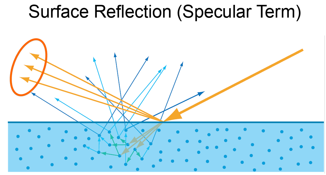
Some of the light reflects off the surface, creating visible highlights. The rest penetrates into the material, where it becomes attenuated due to absorption and scattering within the medium. This process is responsible for effects like subsurface scattering and volumetric absorption, which are essential for rendering realistic materials such as skin, wax, milk, or water.
A common real-world example is holding your finger up to sunlight. You’ll notice a glowing red edge around the silhouette of your finger—this is light scattering beneath the surface of the skin and exiting at different points. It demonstrates how light can enter a translucent material, bounce around internally, and emerge with a diffused, softened appearance. All these are called subsurface scattering.
If the area below picture are smaller than one pixel, then we can treat them as a local point, treating like one particle as shown on next image.
Mathematics
Radiance is a physical quantity that measures the intensity of light traveling along a specific direction — essentially, how much light energy is flowing through a point in a specific direction. In rendering, this typically corresponds to the light that reaches the camera through a pixel along a ray.
Radiance is spectrally varying, meaning it can be described across different wavelengths (or as RGB in discrete form).
The unit of radiance is: W / (m²·sr)
BRDF
The Bidirectional Reflectance Distribution Function (BRDF) defines how light is reflected at an opaque surface. The BRDF is defined as the ratio of the reflected radiance in a specific outgoing direction to the incident irradiance from a specific incoming direction, for given azimuth and zenith angles of both incidence and reflection.
Intuitively, the way a surface appears depends on two things:
The direction of incoming light (where the light is shining from)
The viewing direction (where the camera or eye is positioned)
l represent the light direction, and v as a view direction. If you take a closer look on image below, we can actually calculate how much lights are coming through that patch into one points.
Now, we can truly define the what is really the definition of BRDF. Suppose we are given an incoming light direction ωᵢ (a unit vector pointing toward the surface), and an outgoing/viewing direction: ωₒ (a unit vector pointing away from the surface, typically toward the camera). BRDF can be defined as the ratio of the quantity of relfected light in direction ωₒ, to the amount of light that reaches the surface from direction ωᵢ. Which means, the quqntity of light reflected from the surface in direction ωₒ. Lo, and the amount of light arriving from direction ωᵢ, Ei.
The BRDF is the ratio of the differential outgoing radiance 𝑑𝐿𝑜(𝜔𝑜) in direction 𝜔𝑜 to the differential incoming irradiance 𝑑𝐸𝑖 from direction 𝜔𝑖.
There are two classes of BRDFs and two important properties. BRDFs can be classified into two classes, isotropic BRDFs and anistorpics BRDFs. The two important properties of BRDFs are reciprocity and conservation of energy. Reciprocity states that the BRDF remains unchanged when the directions of incoming and outgoing light are swapped. In other words, the ratio of reflected radiance in one direction to the irradiance from another direction is the same, regardless of whether the directions are reversed:
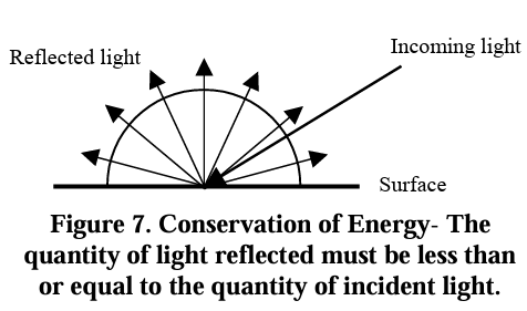
Conservation of energy ensures that the total reflected energy from a surface cannot exceed the total incoming energy. That is, the BRDF must not allow more light to be reflected than is received, ensuring energy is preserved in the system as shown below
Reflectance Equation
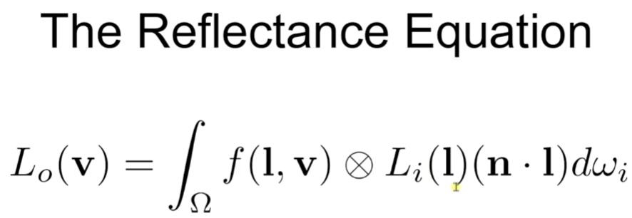
All of the things we cover now reveal as one equation called reflectance equation. Outgoing Radiance from a point equals to the integral of incoming radiance times BRDF times the sign Factor over the hemisphere of incoming directions. Note that it is component-wise RGB multiplication. In detail, Lo is basically what we want to calculate in the pixel shader. Li(l) is the amount of incoming light (RGB). ndotl is the factor that increase and decrease the light power. f(l,v) is the BRDF term, then we integral all that terms. Unit-wise, Lo(V) is RGB, f(l,v) is RGB, Li(l) is also RGB with scalar. So output must be RGB.
Microfacet Theory
To achieve a visually immersive experience, both the diffuse and specular components of light reflection are important. Let’s begin by examining the specular term.
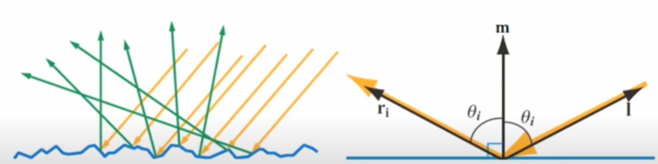
Microfacet Theory provides a framework for modeling surface reflection on rough or non-optically-flat surfaces. Rather than treating a surface as perfectly smooth, it assumes the surface is composed of many tiny, flat facets—each acting like a perfect mirror. Depending on the surfaces, BRDFs output term can be varied.
By zooming in on a small surface region, we approximate it as a collection of microscopic facets, each with its own orientation. At any given point, light may be reflected or refracted depending on the orientation of the microfacets. This interpretation allows us to derive realistic BRDFs that account for the surface roughness and the distribution of microfacet normals.
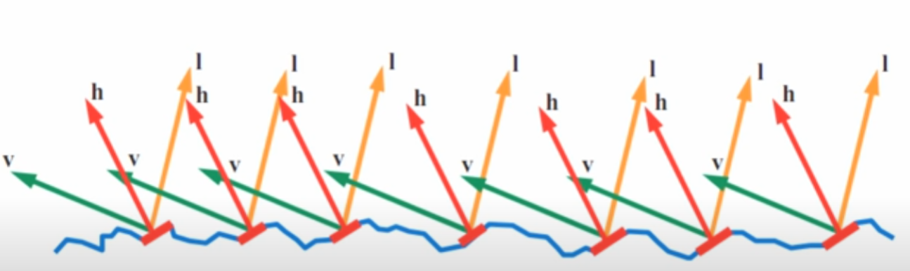
The half vector is simply the direction that the microfacets must be aligned with in order to reflect light from the light direction L into the view direction V.
In other words, the proportion of light that is reflected from L to V depends on how many microfacets have their surface normals aligned with this half vector. These microfacets act like tiny mirrors that perfectly reflect light when their normals match the half vector. The more microfacets oriented in the direction of H, the stronger the specular reflection in the view direction V. This is basically halfway vector calculation in phong model.
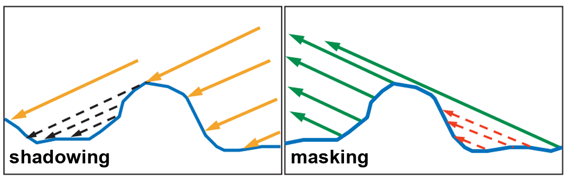
Depending on the surface geometry, not all microfacets aligned with the half vector can contribute to reflection. For example, if a nearby facet is taller and blocks the incoming light from reaching a microfacet, this is known as shadowing. On the other hand, if the reflected light from a microfacet is blocked in the direction of the viewer, this is referred to as masking. In reality, the some light can reach into shadow area, but Micro BRDFs ignore all that.
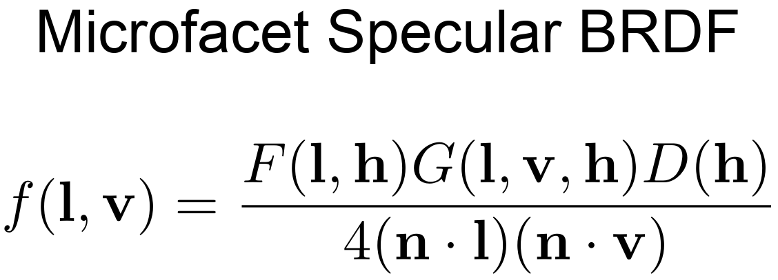
Microfacet Specular BRDF
This is the general form of Microfacet Specular BRDF.
F(l,h) is Fresenel Reflectance. This basically show depending on the view direction(incident angle) and surface normal, and the RoI. The vale of frasnel can be varied as shown below.
Since the barely change parts is kind of like a starting point (parameter), so that we can tweak them from there. The image below shows each fresnel value for each metal and dielectric.
The speaker mentioned that Schlick Approximiation is good enough to implement.
The normal distribution D(h), describes how densely microfacet normals are aligned with a given half-vector direction h. In simple terms, it tells us how many microfacets are oriented in a way that would reflect light from the incoming direction L toward the outgoing view direction V. Since perfect specular reflection happens only when the microfacet normal matches the half-vector (the vector halfway between light direction L and view direction V), D(h) essentially controls the shape and sharpness of the specular highlight. You can actually see all those functions in Cook-Torrance
Finally, the geometry function, often denoted as G(l, v, h), accounts for shadowing and masking effects caused by the microgeometry of a surface. Shadowing occurs when incoming light (from direction l) is blocked by parts of the surface before it can reach a microfacet. Masking happens when the reflected light (toward the view direction v) is blocked by other parts of the surface, preventing it from escaping.
So, G(l, v, h) tells us how much of the microfacet reflection is actually visible, based on how the surface self-occludes due to its roughness.
The image below is commonly used, smith function, to illustrate the concept of the geometry function, as it has been both mathematically and physically validated:
Putting It All Together
D(h) (Normal Distribution Function): Describes how many microfacets are oriented in the direction of the half-vector h, which is the direction needed to reflect light from L to V. It essentially tells us how aligned the surface microfacets are with the ideal reflection direction.
F (Fresnel Term): Tells us how reflective each of those microfacets are, depending on the viewing angle and material properties.
G(l, v, h) (Geometry Function): Tells us how many of those microfacets are visible and not occluded, meaning they can actually participate in reflecting light from the light direction L to the view direction
In physically based rendering (PBR), we often split surface reflection into diffuse and specular components. The diffuse term accounts for the light that enters a surface, scatters beneath it, and then exits in a different direction.
Lambertian Diffuse Model assumes light is scattered equally in all directions, and the surface looks the same from all viewing angles. Fairly simple and works well for matte surfaces like a paper.
Diffuse BRDF (Lambert): 𝑓𝑑 = C𝑑 / 𝜋, where the C𝑑 is the diffuse color. In real world, the rougher surfaces doen’t scatter light perfectly evenly. For example, skin, cloth have subsurface scattering and edge darkening. A specular reflection becomes sharper, the diffuse should became broader (vice versa). Thus Lambertian diffuse isn’t always phsycially accurate when the rough microfacet is applied.
The speaker also mentioned that Diffuse Roughness = Specular Roughness. It’s because of the assumption. “If the surface is rough for specular, it must also be rough for diffuse” but the assumption is wrong because specular roughness comes from surface microgeometry, and diffuse roughness is caused by the subsurface scattering, material properties, and light diffuion inside the medium..
Results
Of course, this is a summary based on content from SIGGRAPH and various other sources, so it might not be perfect or comprehensive. However, I thought it would be helpful for the understanding stage, so I put together a blog post to organize the information.
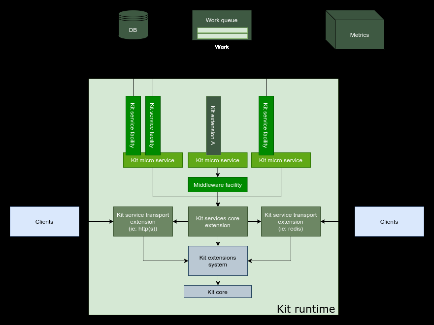
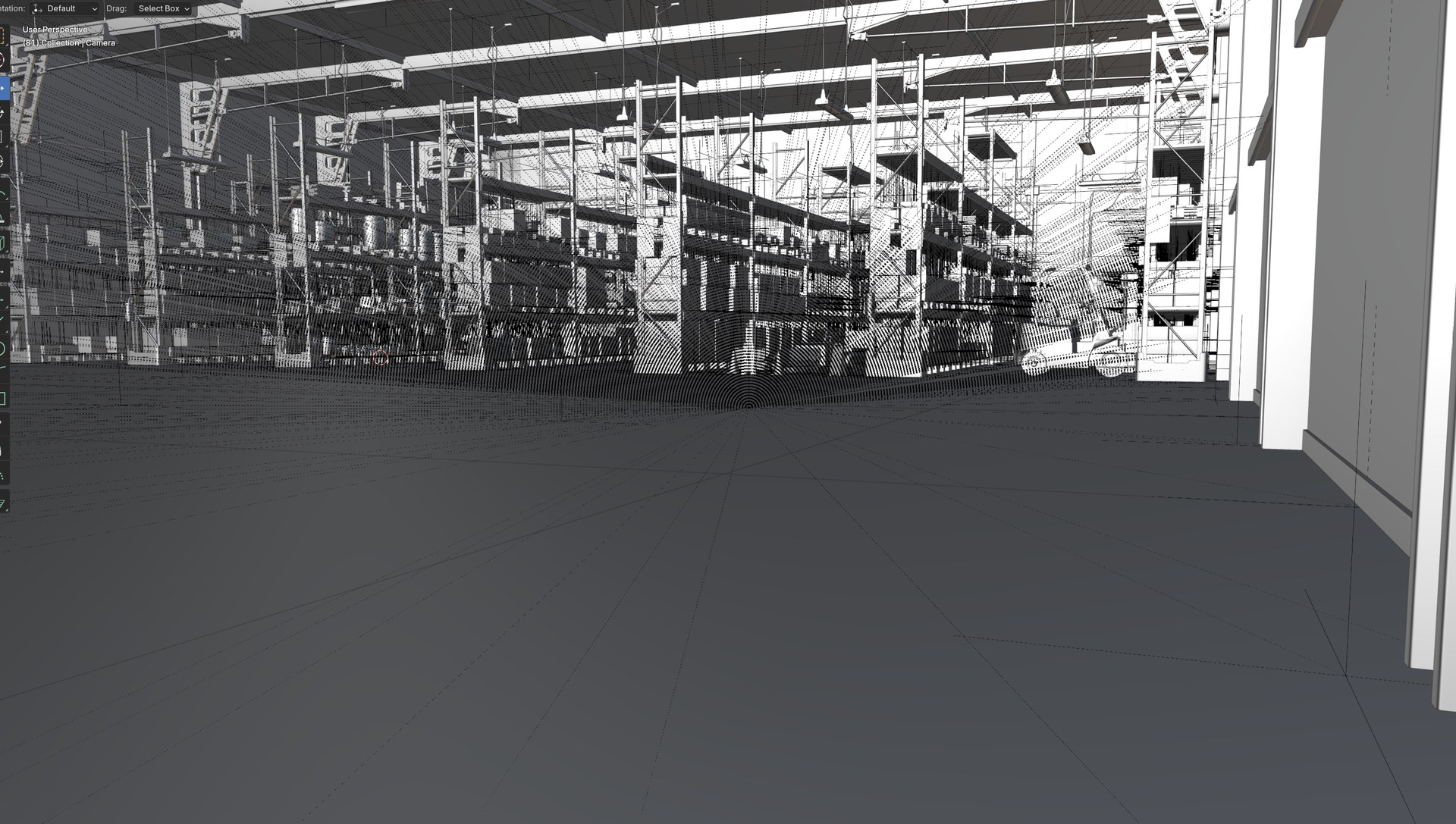
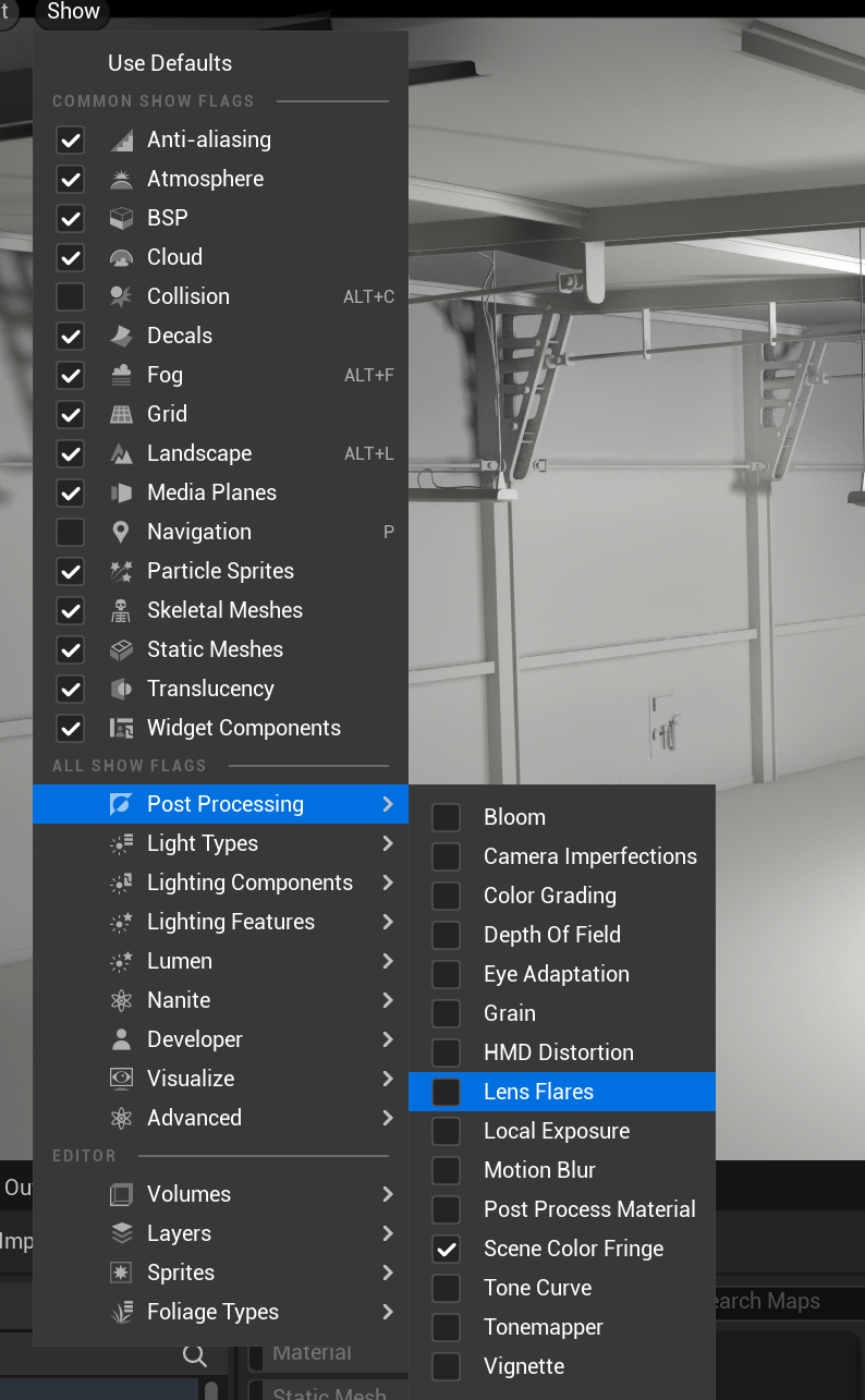
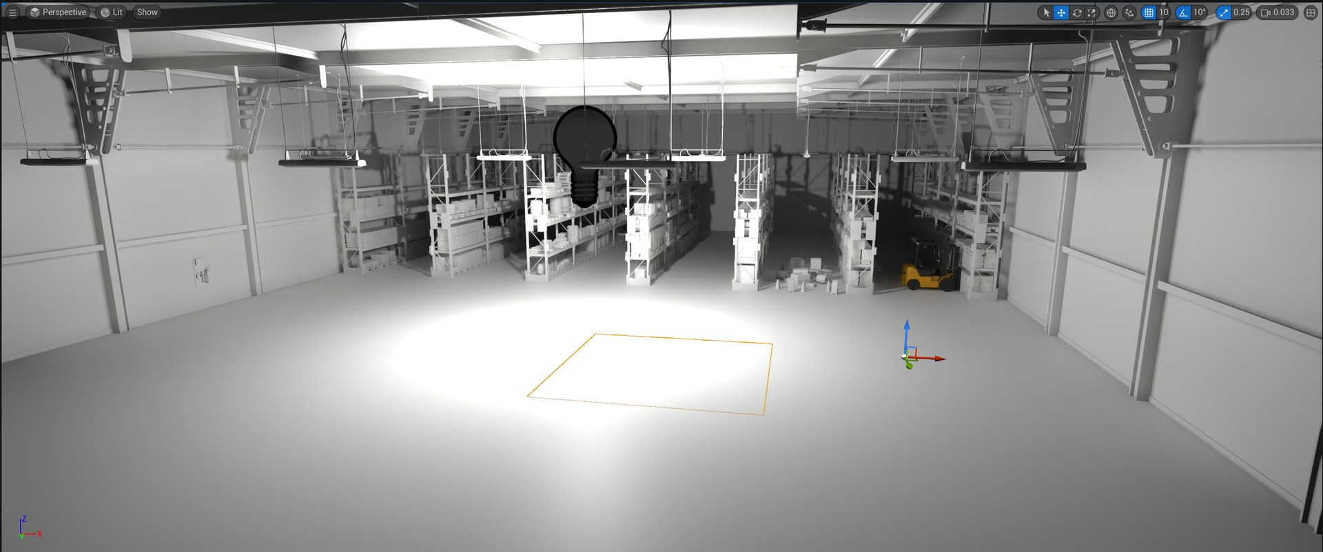
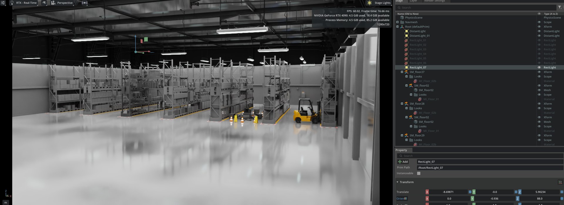
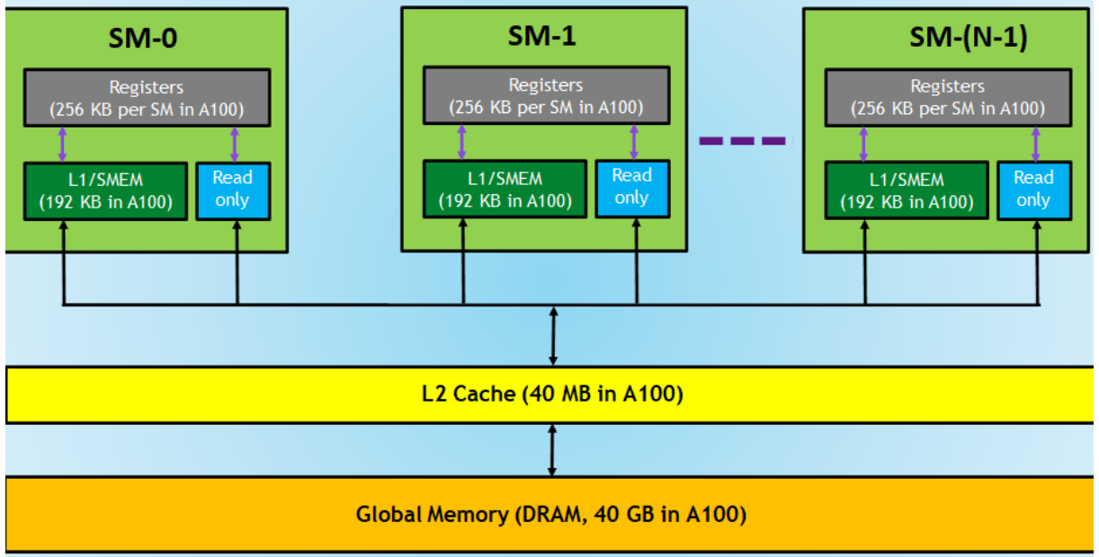
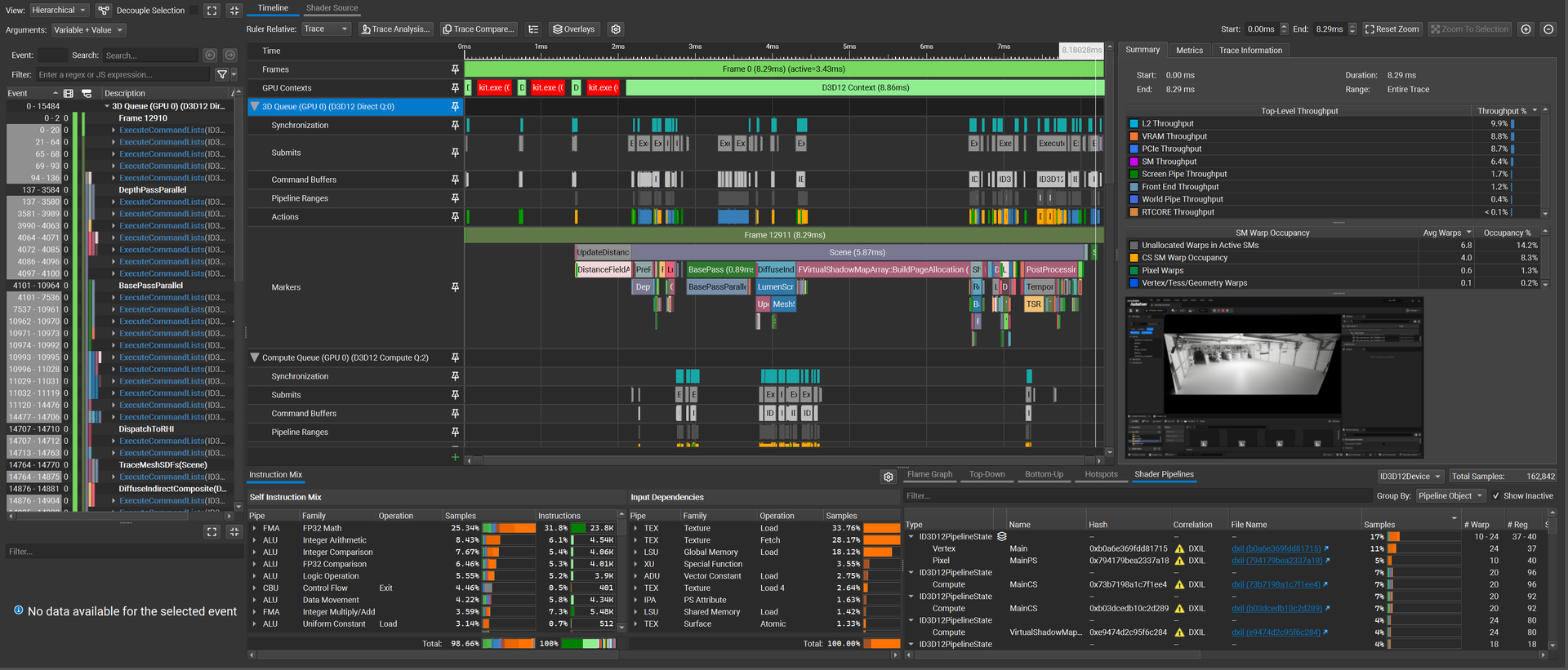
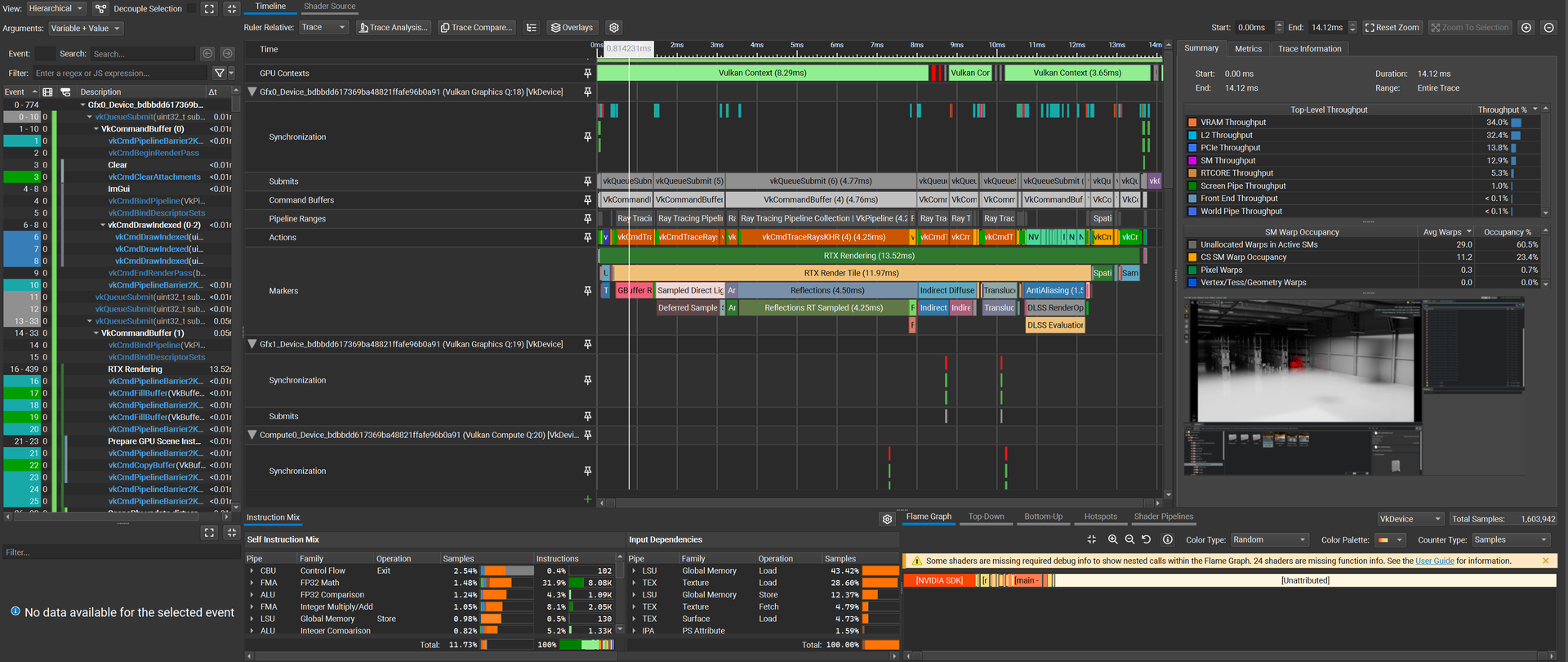
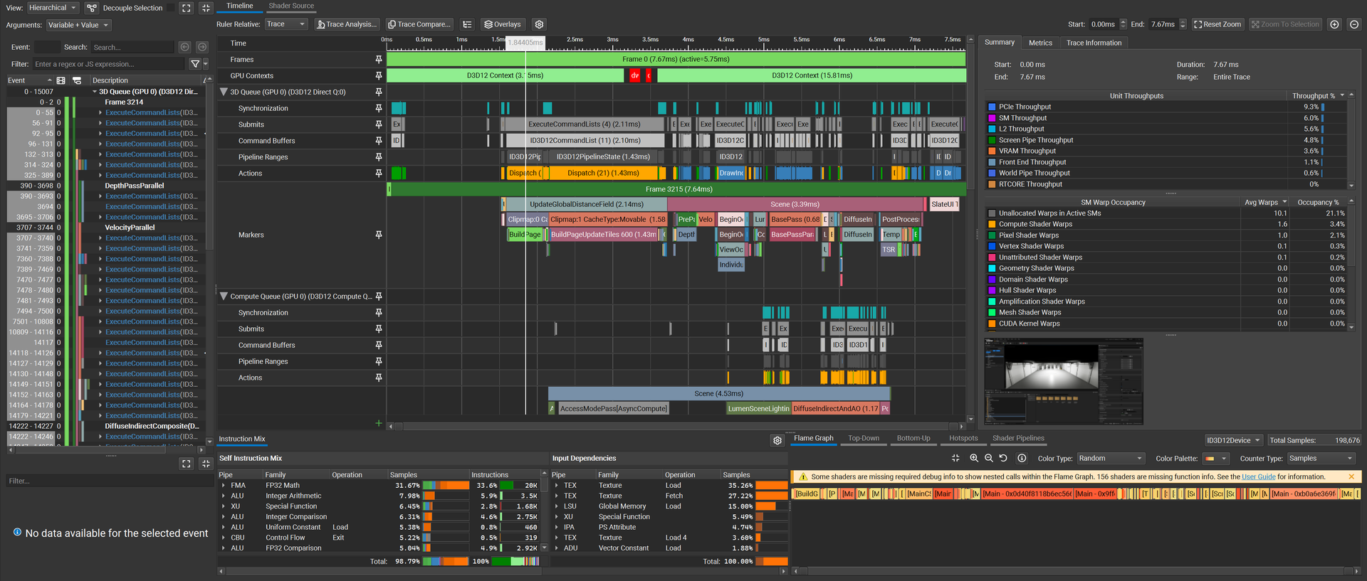
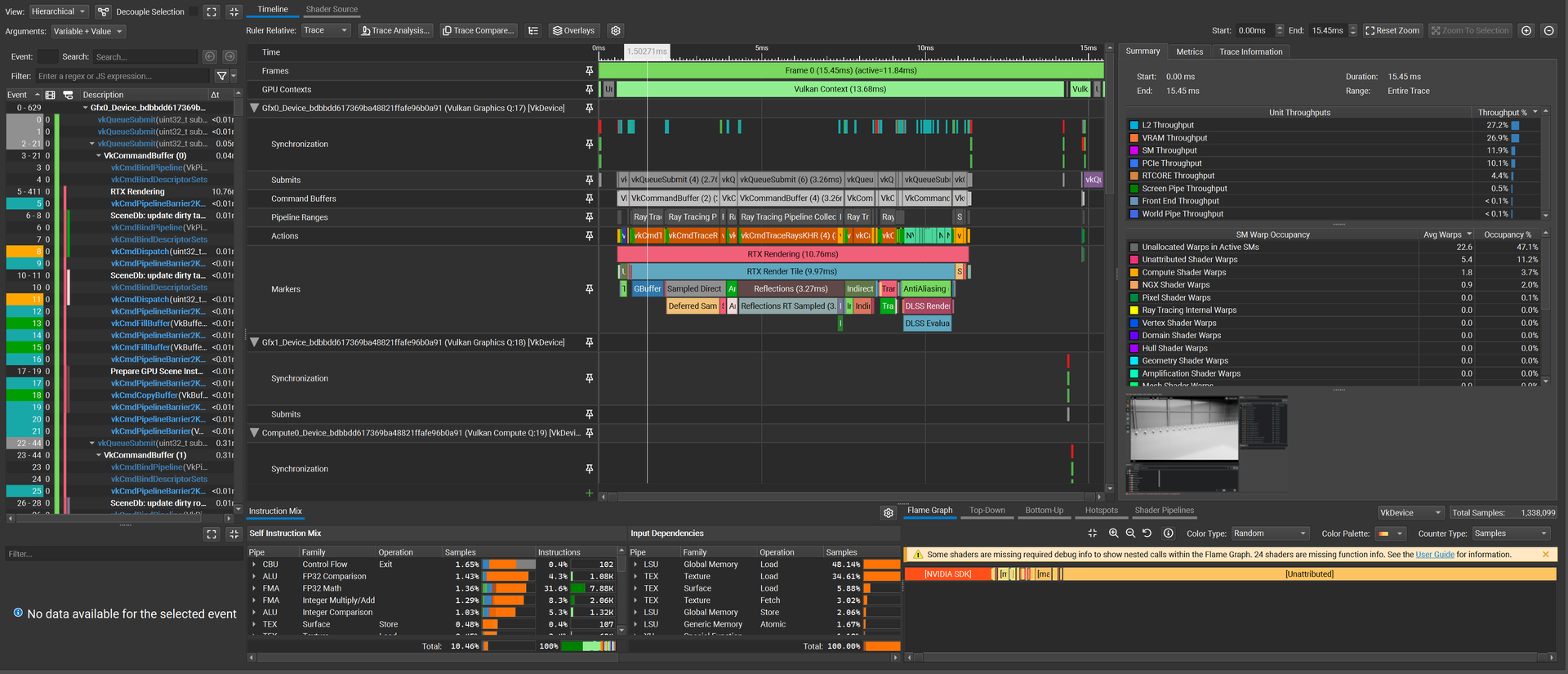
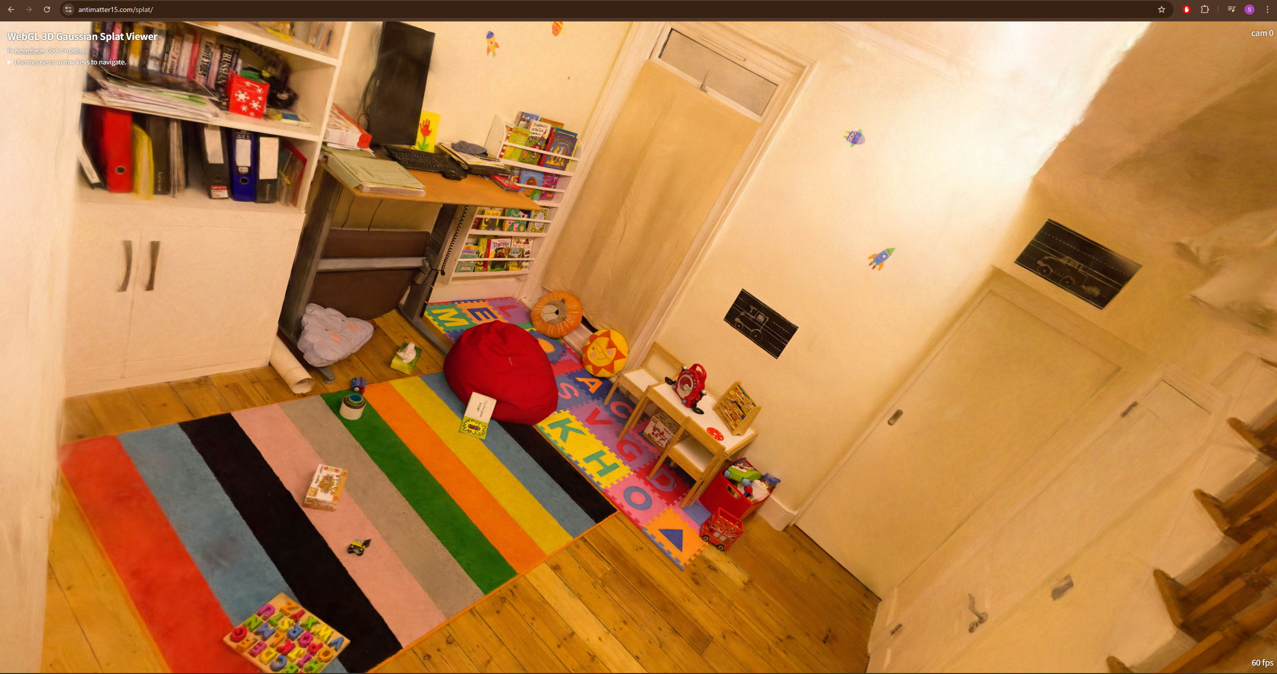
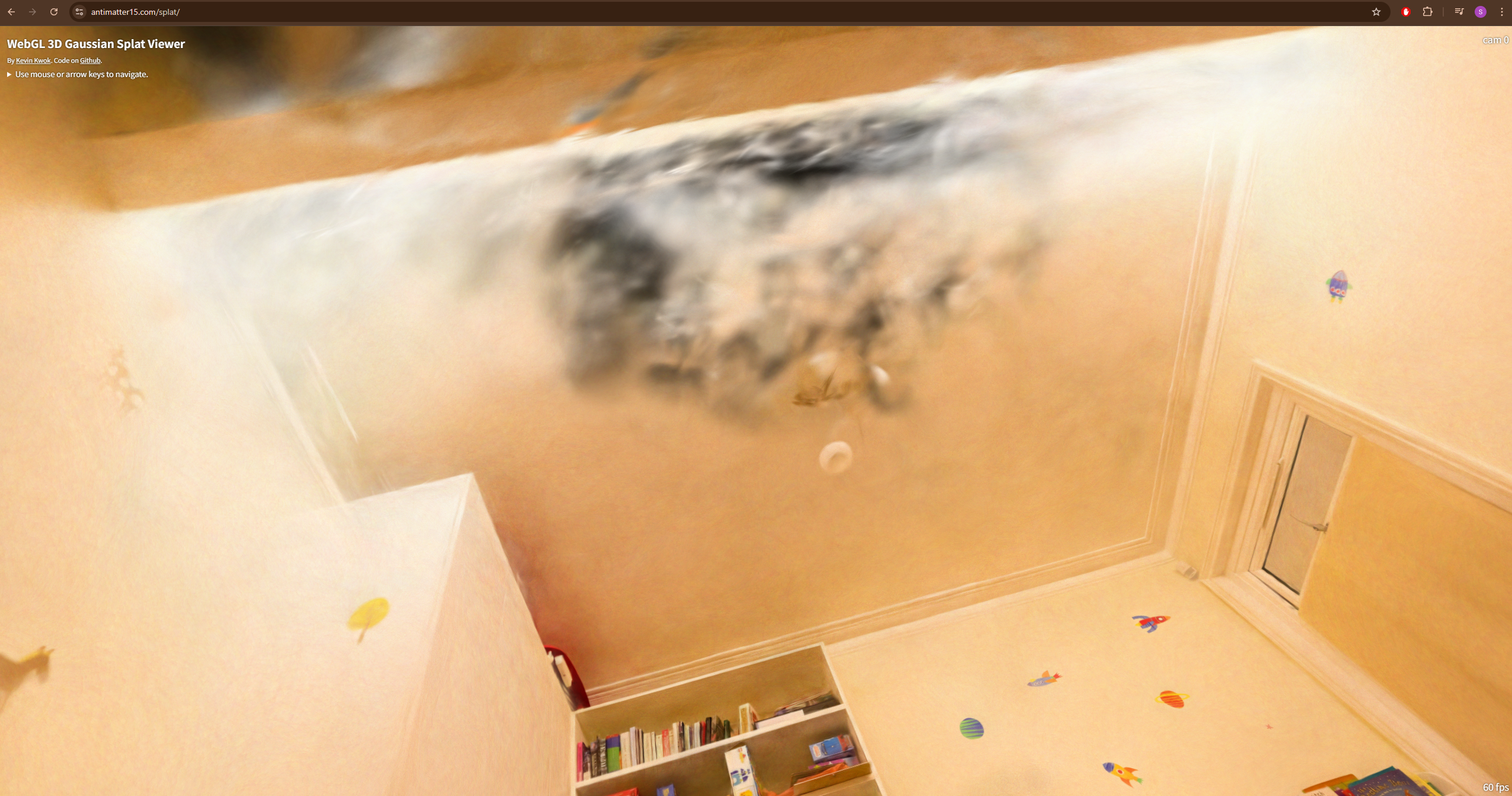
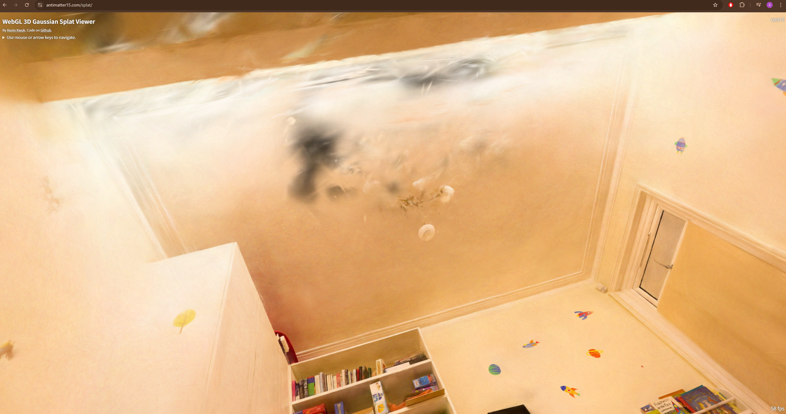
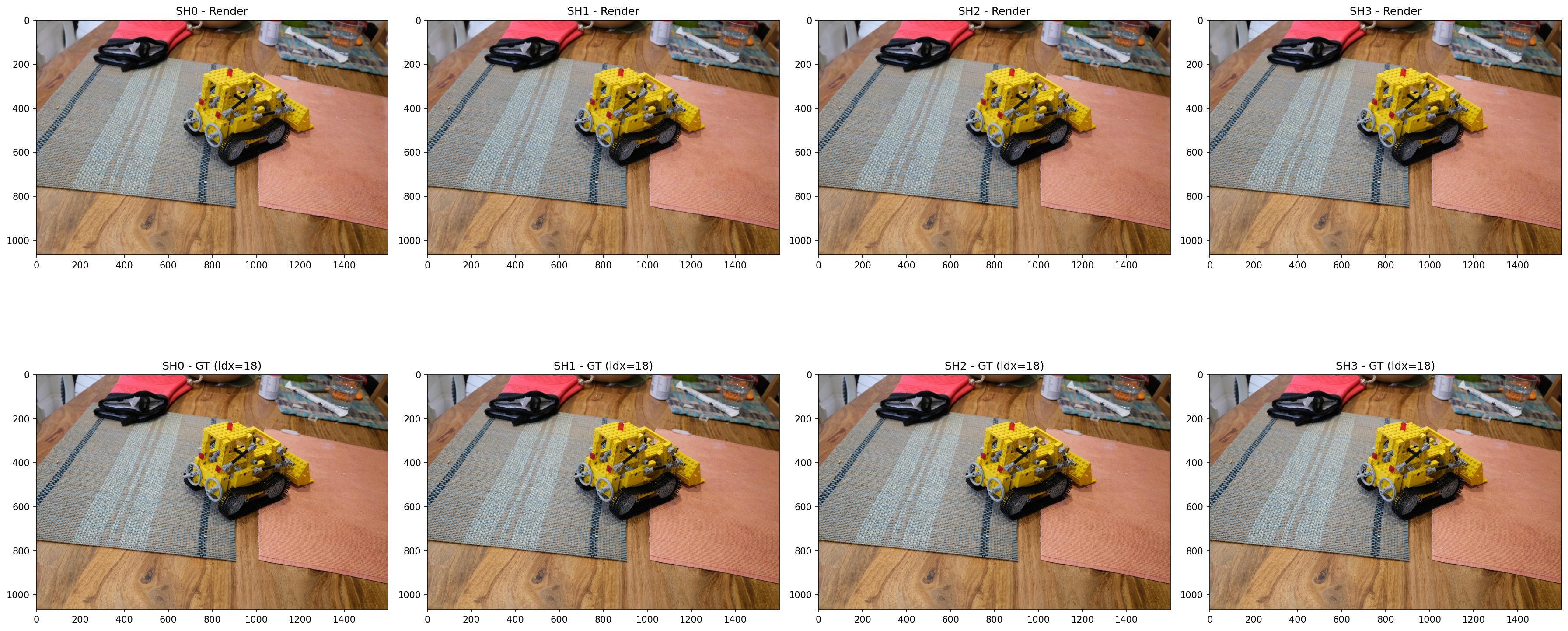
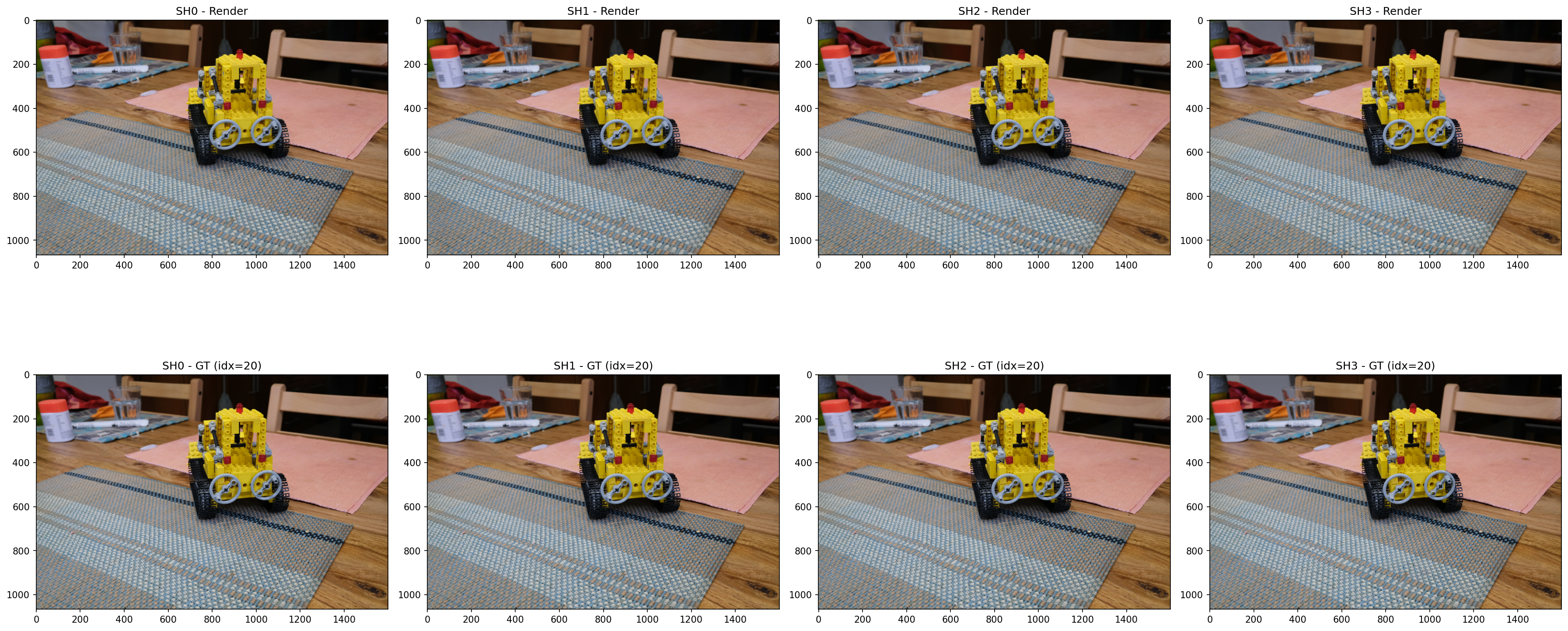
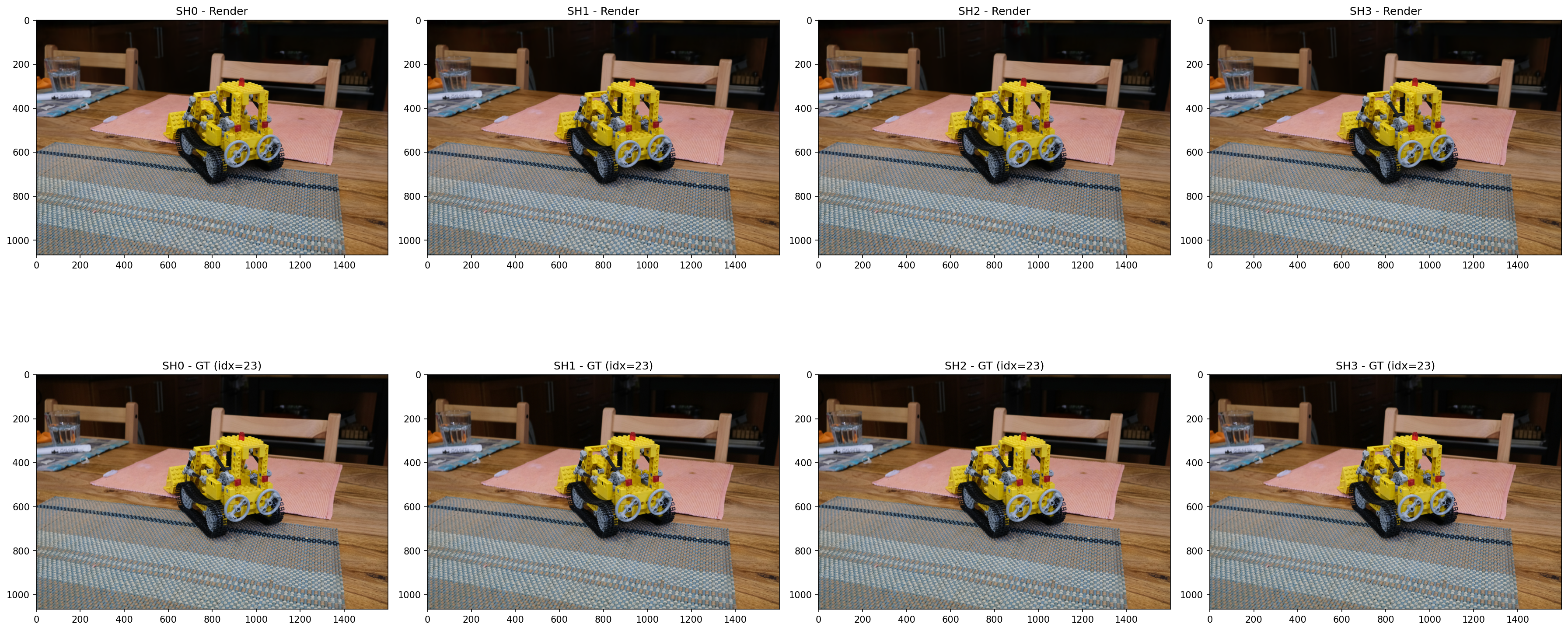
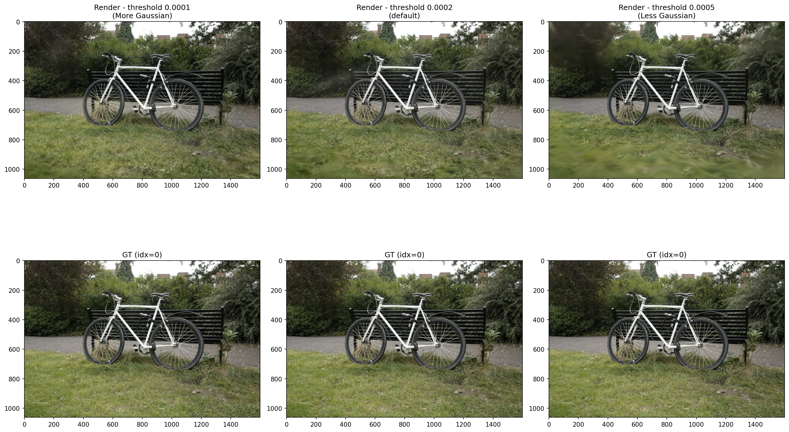
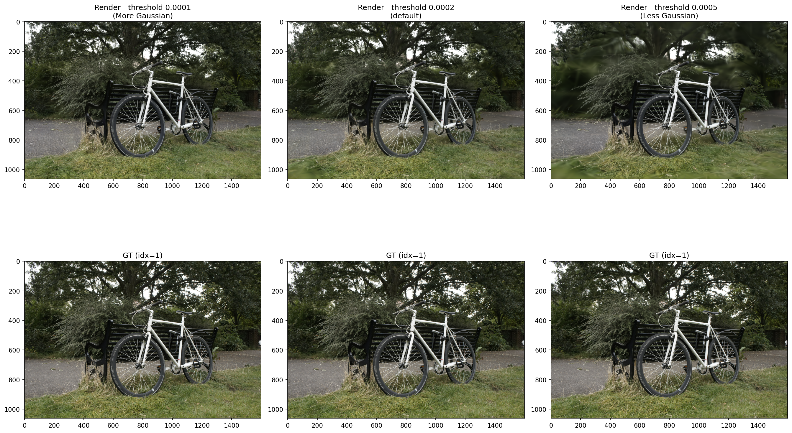
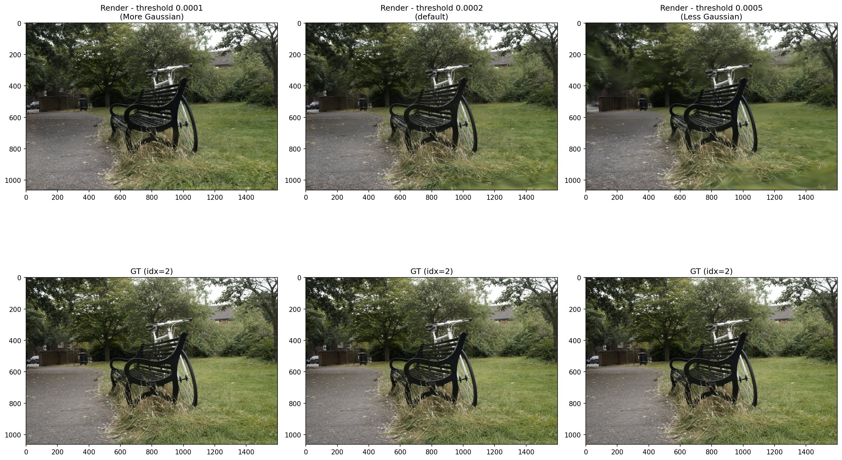
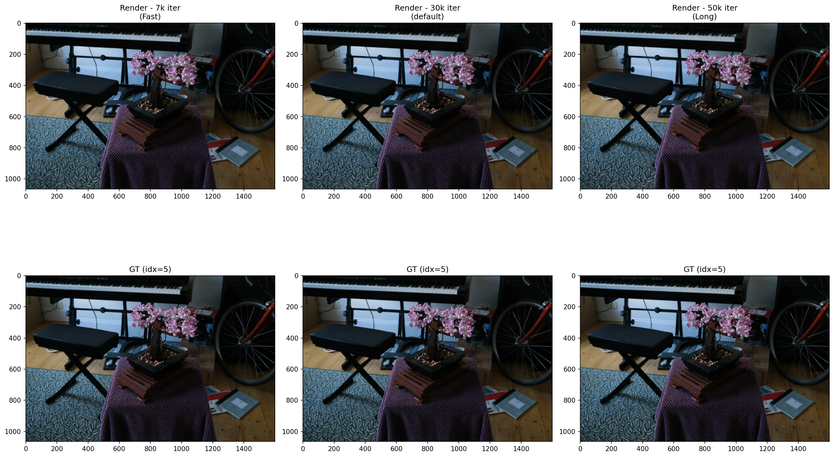
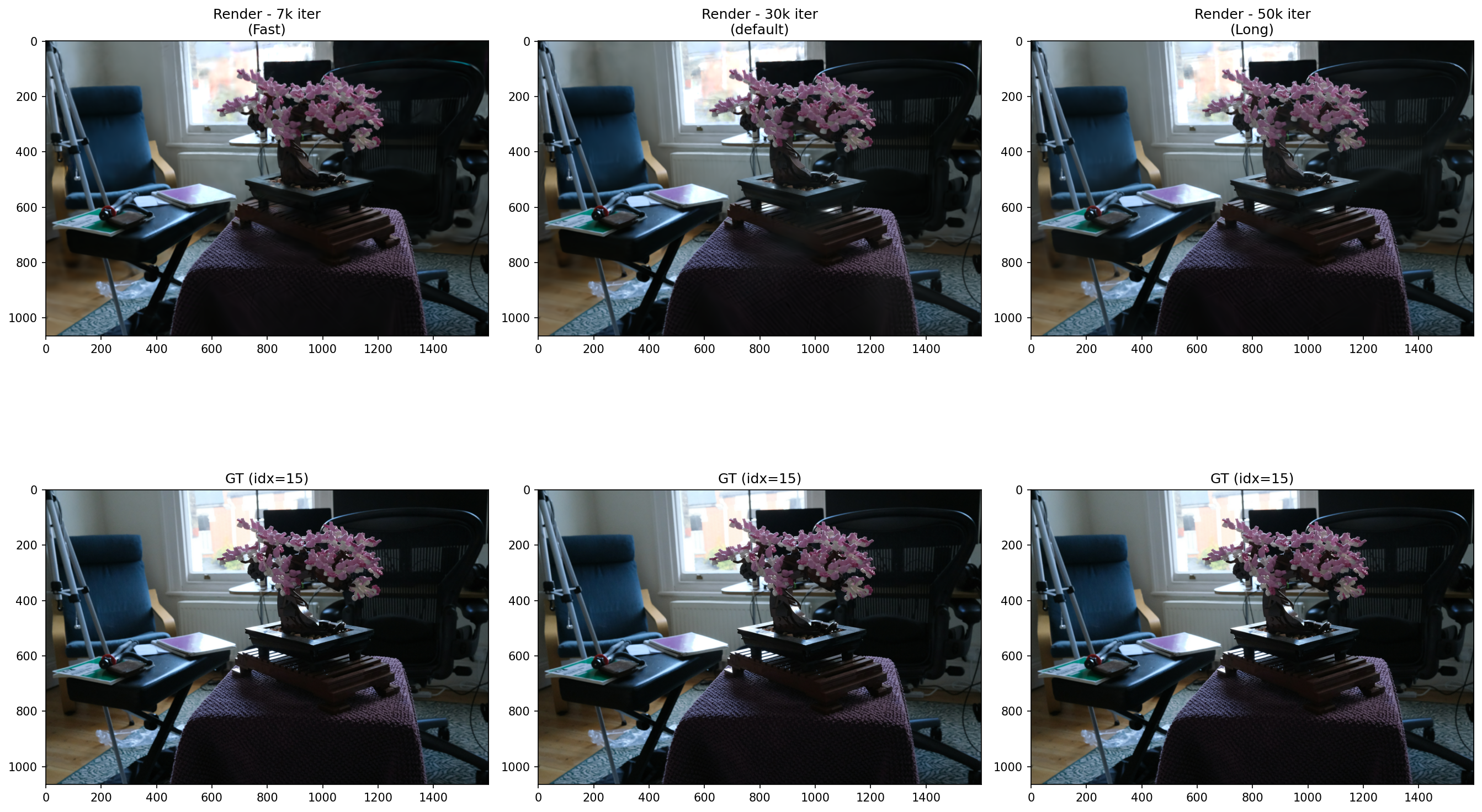
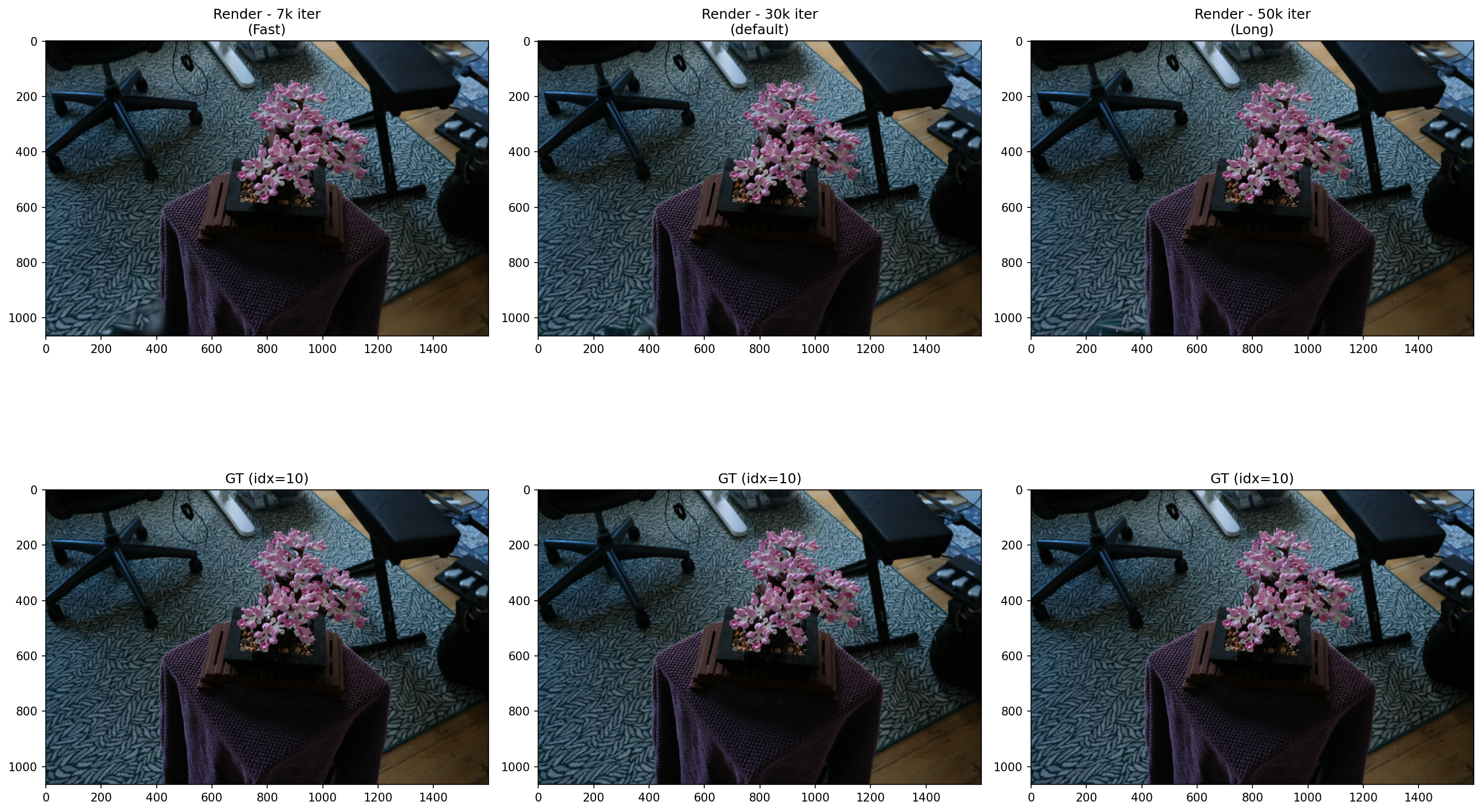
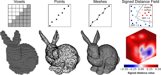
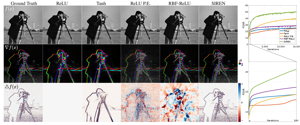
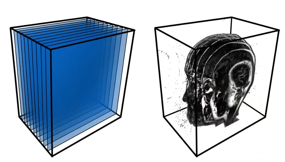
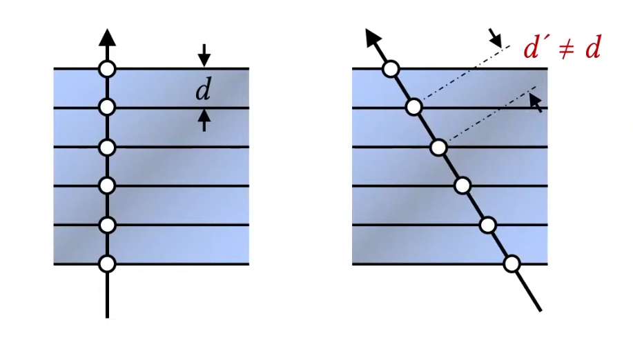
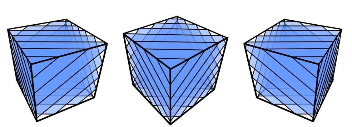
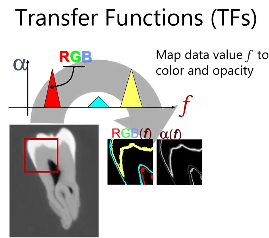
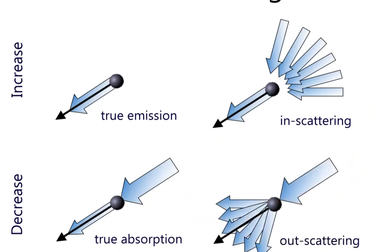
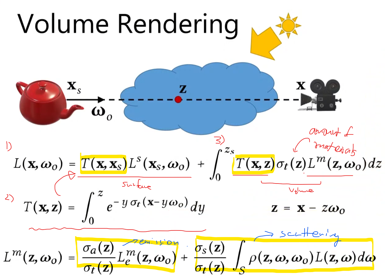
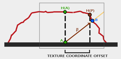
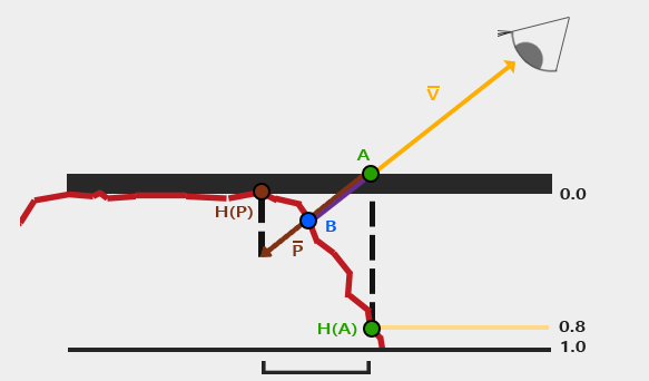
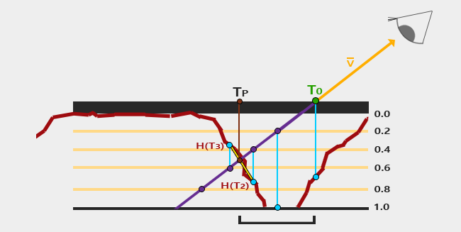
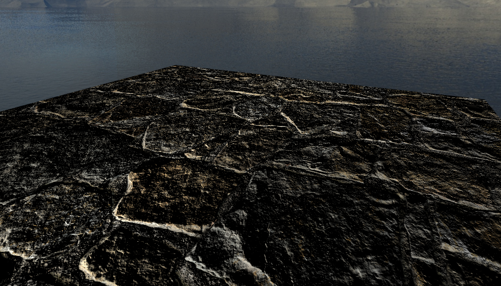
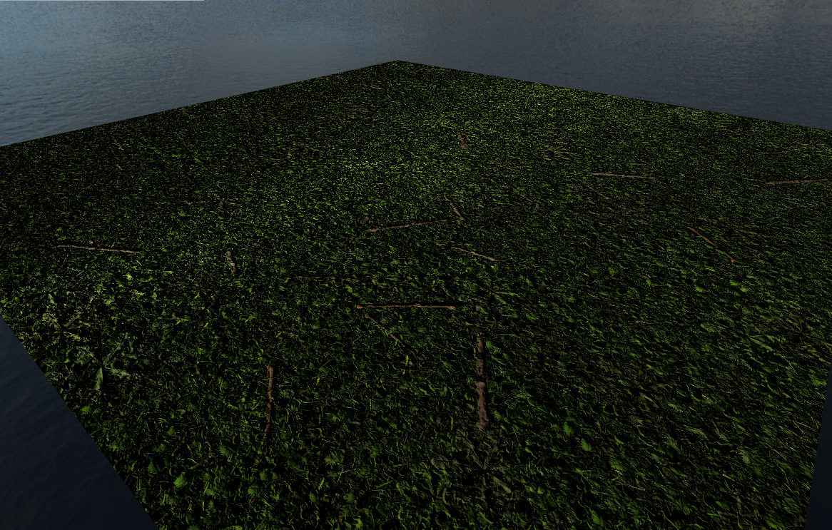
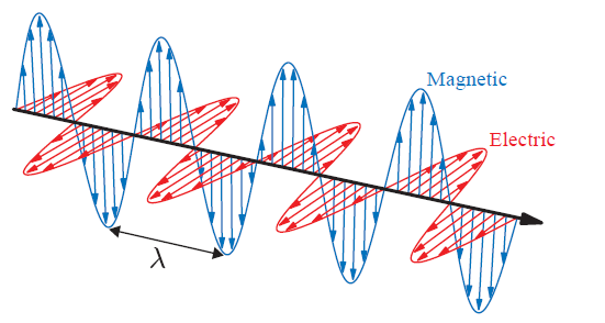
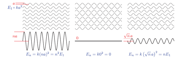
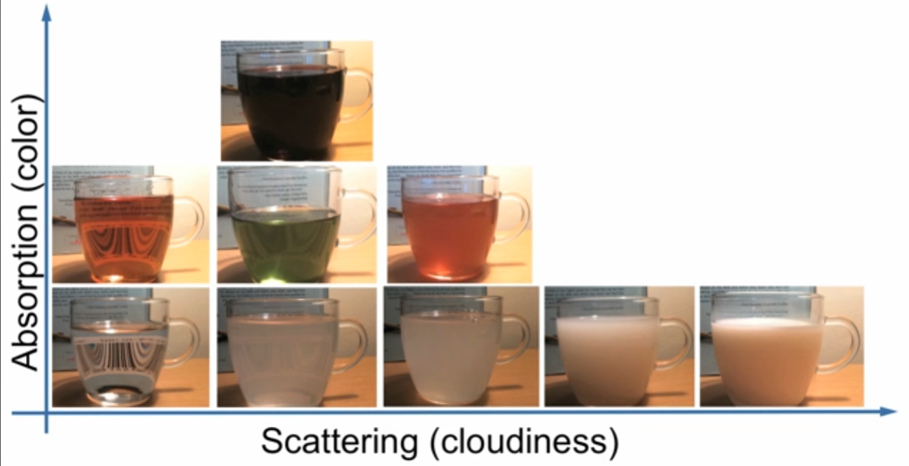
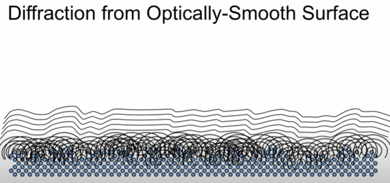
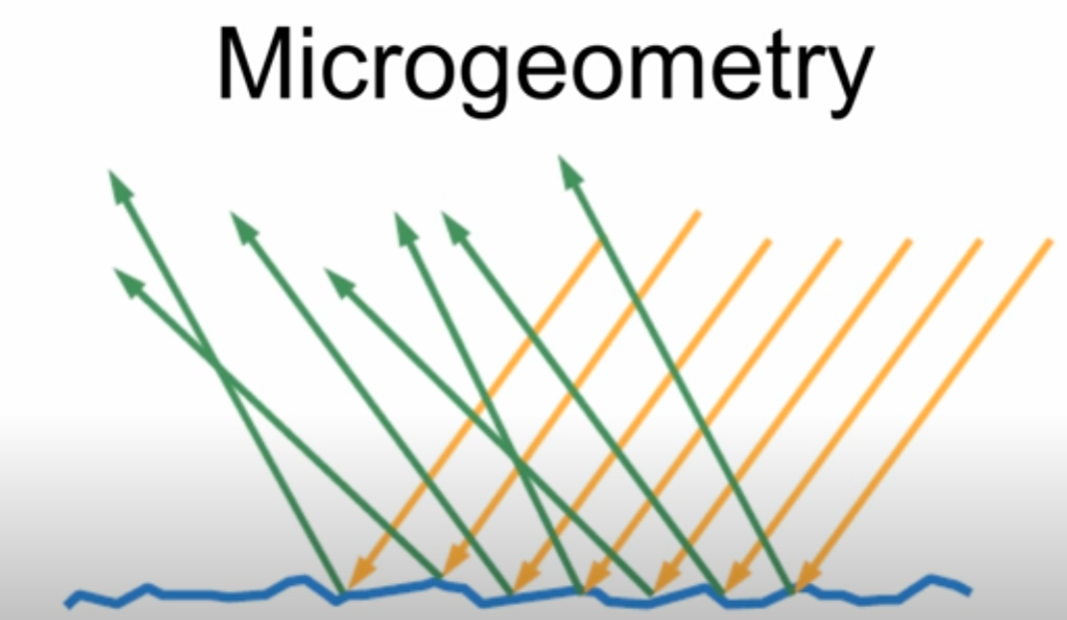
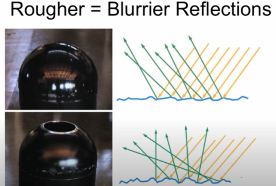
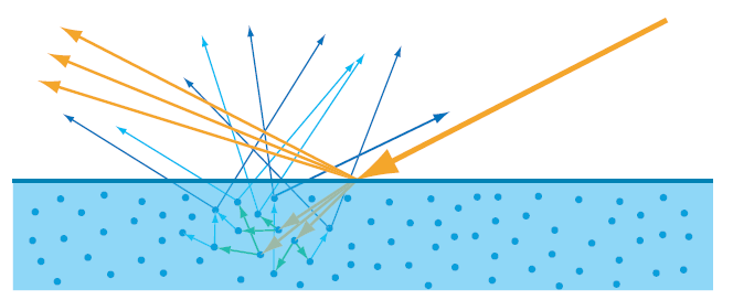
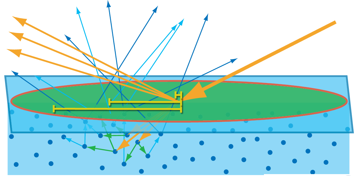
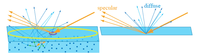
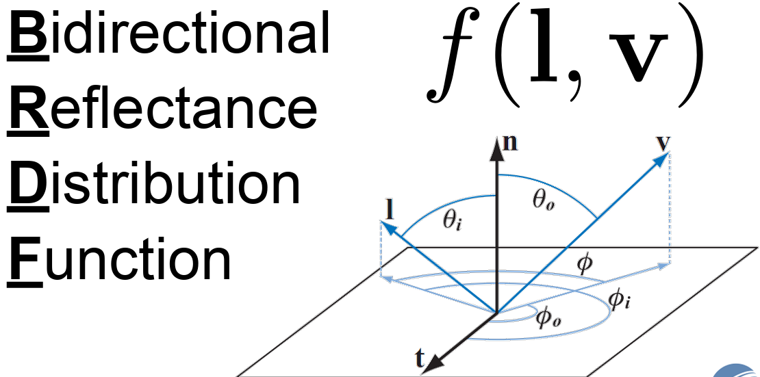

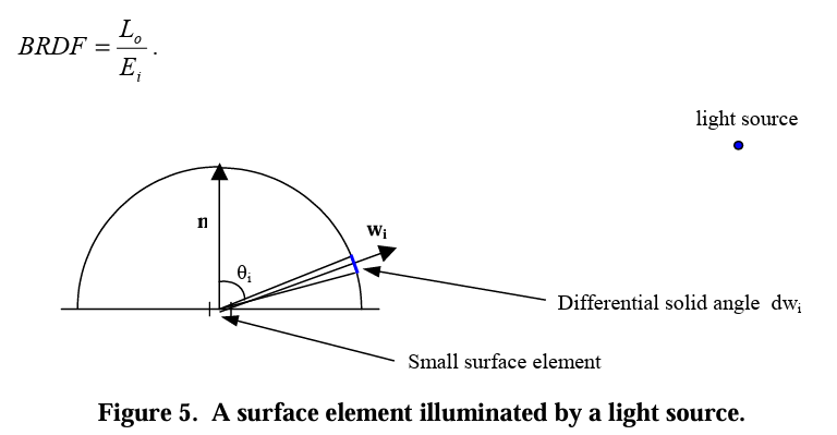 \[f_r(\omega_i, \omega_o) = \frac{dL_o(\omega_o)}{dE_i(\omega_i)}\]
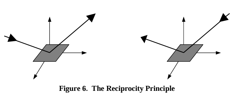 \[\text{BRDF}_{\lambda}(\theta_i, \phi_i, \theta_o, \phi_o) = \text{BRDF}_{\lambda}(\theta_o, \phi_o, \theta_i, \phi_i)\]