• Reviewing what I studied, how this work will be explained as well.

Introduction

As we saw with Dijkstra’s and Bellman-Ford algorithms, we need to check if DP can be applied by identifying optimal substructure and overlapping subproblems. In the context of shortest paths, a portion of a shortest path is itself a shortest path, and overlapping subproblems occur when we reuse partial shortest paths. The approach involves finding three nodes u, v, and k where the path from u to v becomes shorter by going through k.

The key difference between Floyd-Warshall and the other two algorithms is that Floyd-Warshall isn’t fixed to a single starting vertex - it finds the shortest paths between all pairs of vertices. While the algorithm proceeds in stages based on intermediate nodes, it doesn’t require finding the unvisited node with the minimum distance at each step. Due to the graph’s characteristics, Floyd-Warshall can be implemented using an adjacency list, but it’s typically implemented with an adjacency matrix. This makes a bottom-up approach quite feasible.

Recurrence Relation:

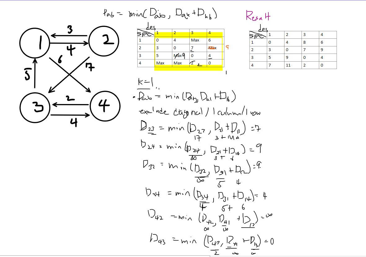
Being able to solve a problem with Dynamic Programming means we can define a recurrence relation. At each step, we check if going through a specific node k provides a shorter path. We compare the direct path a->b with the path a->k->b:

Dab = min (Dab, Dak + Dkb) 이런식으로 세울수 있다.

Let’s look at an example using this recurrence relation. The right side shows the graph being updated when k = 1. By applying this process for each node k, we can see the final result in the upper right of the algorithm.

we can infer that the time complexity will be O(n³).

Implementation

코드를 확인해보자…

constexpr double kInf = numeric_limits<double>::infinity();
vector<vector<double>> graph =
{
	{0.0, 3.0, 8.0, kInf, -4.0},
	{kInf, 0.0, kInf, 1.0, 7.0},
	{kInf, 4.0, 0.0, kInf, kInf},
	{2.0, kInf, -5.0, 0.0, kInf},
	{kInf, kInf, kInf, 6.0, 0.0}
};

void FloyedWarshall(const vector<vector<double>>& graph) {
    vector<vector<dobule>> dist = graph;
    int V = graph.size();

    // The graph is already initialized above
    // If not, diagonal values should be 0 and other indices
    // should be filled with appropriate values
    for (int k = 0; k < V; k++) {
        auto dist_k = dist;

        for(int i = 0; i < V; i++) {
            for(int j = 0; j < V; j++) {
                if (dist[i][k] + dist[k][j] < dist[i][j]) {
                    dist_k[i][j] = dist[i][k] + dist[k][j];
                }
            }
        }
    }
}

The implementation is surprisingly simple. We perform updates when necessary. Here’s a Python implementation which might be more straightforward, though it differs in indexing:

INF = int(1e9)

node = int(input())
edge = int(input())
graph = [[INF] * (n+1) for _ in range(n+1)]

for a in range(1, n+1):
    for b in range(1, n+1):
        if a == b:
            graph[a][b] = 0

for _ in range(edge):
    a, b, c = map(int, input().split())
    graph[a][b] = c

for k in range(1, n+1):
    for i in range(1, n+1):
        for j in range(1, n+1):
            graph[i][j] = min(graph[i][j], graph[i][k] + graph[k][j])

To summarize, the Floyd-Warshall algorithm has a time complexity of O(n³).

Resource

• FloydWarshall Algorithm

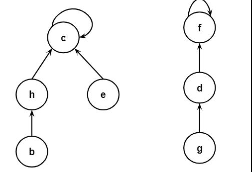
Cycle detection in a directed graph is a fundamental problem in graph theory with applications in deadlock detection, dependency resolution, and circuit analysis. The algorithm I’ve implemented uses a depth-first search (DFS) approach with a recursive traversal strategy to identify cycles in directed graphs.

Key Concepts

The algorithm relies on three key data structures:

1. A visited flag for each vertex to track which vertices have been explored
2. An on_stack array to track vertices currently in the DFS recursion stack
3. An edge_to array to maintain the DFS tree structure for cycle reconstruction

Implementation

struct Vertex 
{
    Vertex(int v) { index = v; }

    int index = -1;
    bool visited = false;
    vector<Vertex*> out_neighboors;
}

class Graph
{
public:
    Graph(int num_vertices)
    {
        vertices.resize(num_vertices);
        for (int i = 0; i < num_vertices; i++)
            vertices[i] = new Vertex(i);
    }

    ~Graph() 
    {
        for (auto* v : vertices)
            delete v;
    }

    void addEdge(int v, int w)
    {
        verticies[v]->out_neighboors.push_back(vertices[w]);
    }

    void DetectCycle()
    {
        on_stack.resize(vertices.size(), false);
        cycle.clear();
        edge_to.resize(vertices.size(), nullptr);

        for (auto* v : vertices)
            v->visited = false;

        for (auto* v : vertices)
        {
            DetectCycleRecurr(v)
            if (!cycle.empty()) {
                cout << "cycle Detected" << endl;
            }
        }
    }

    void DetectCycleRecurr(Vertex* v)
    {
        v->visited = true;
        on_stack[v->index] = true;

        for(auto* w : v->out_neighboors)
        {
            if (!cycle.empty())
                return;
            else if (!w->visited) 
            {
                edge_to[w->index] = v;
                DetectCycleRecurr(w);
            }
            else if (on_stack[w->index])
            {
                Vertex* x = v;
                cycle.push_back(x);

                while(x->index != w->index) 
                {
                    cycle.push_back(x);
                    x = edge_to[x->index]
                }

                reverse(cycle.begin(), cycle.end())
                return;
            }
        }
    }

private:
    vector<Vertex*> vertices;
    vector<Vertex*> cycle;
    vector<bool> stack;
    vector<Vertex*> edge_to;
}

int main() 
{
    Graph g(3);
    g.addEdge(0, 1);
    g.addEdge(1, 2);
    g.addEdge(2, 0);
}

Time Complexity

Time Complexity: O(V + E) where V is the number of vertices and E is the number of edges. Each vertex and edge is processed exactly once in the worst case

The cycle reconstruction takes at most O(V) time

Space Complexity: O(V)

on_stack, edge_to, and recursion stack each require O(V) space. The cycle array stores at most V vertices

• Reviewing what I studied, how this work will be explained as well.

The Bellman Ford Algorithm is a graph search algorithm that finds the shortest path from a source vertex to all other vertices in a weighted graph. It is similar to Dijkstra’s Algorithm but can handle graphs with negative weight edges. However, it can detect negative cycles, which are cycles whose total weight is negative.

Key Differences from Dijkstra’s Algorithm

1. Negative Weight Edges: Bellman Ford can handle negative weight edges, whereas Dijkstra’s Algorithm assumes all edges have non-negative weights.
2. Negative Cycles: Bellman Ford can detect negative cycles, which is not possible with Dijkstra’s Algorithm.

Algorithm Overview

1. Initialization: Initialize the distance to the source vertex as 0 and all other vertices as infinity.
2. Relaxation: Relax the edges repeatedly. For each edge, if the distance to the destination vertex can be reduced by going through the current vertex, update the distance.
3. Negative Cycle Detection: After relaxing all edges V-1 times, check for negative cycles by attempting one more relaxation. If any distance can still be reduced, a negative cycle exists.

Time Complexity

The time complexity of the Bellman Ford Algorithm is O(V*E), where V is the number of vertices and E is the number of edges. This is because in the worst case, we relax all edges V-1 times.

Implementation

Here’s a corrected and complete implementation of the Bellman Ford Algorithm:

void Print(vector<double>& dist)
{
	for (int i = 0; i < dist.size(); i++)
		cout << setw(6) << dist[i];
	cout << endl;
}

struct Edge
{
	int v, w;
	double weight;
};

constexpr double kInf = numeric_limits<double>::infinity();
vector<double> dist(V, kInf);
for (int v = 1; v < V; v++)
{
	for (auto e : edges)
	{
		if (dist[e.w] > dist[e.v] + e.weight) {
			dist[e.w] = dist[e.v] + e.weight;
			prev[e.w] = e.v;
		}
	}
	Print(dist);
}

Then how do you think about getting the negative edges!? It’s basically same logic! if the distance the next edge is greater than the current(whole) distance, then we can conclude that there will be negative edge. Normally, the dist arrays two indices where negative values are very likely that it’s negative cycle.

Resource

• C++ Data Structures and Algorithm Design Principles: Leverage the power of modern C++ to build robust and scalable applications

• Reviewing what I studied, how this work will be explained as well.

Rod Cutting Problem is a problem that we have a rod of length n and we want to cut the rod into n pieces, and we want to maximize the profit. For example, let’s look at the table below. If I have a rod of length 4, then we have 4 ways to cut the rod. Then we calculate the profit for each case

1. Cut the rod into 1, 1, 1, 1 => max profit = 1 + 1 + 1 + 1 = 4
2. Cut the rod into 2, 2 => max profit = 5 + 5 = 10
3. Cut the rod into 3, 1 or 1, 3 => max profit = 8 + 1 = 9
4. Length 4 rod itself => max profit = 9

the maximum profit we can get is 10.

Length:                     0  1  2  3  4   5   6   7   8   9  10
vector<int> price_table = { 0, 1, 5, 8, 9, 10, 17, 17, 20, 24, 30 };

So, let solve this in naive recursive way

int RecurCutRod(const vector<int>& prices, int length)
{
	if (length == 0)
		return 0; // return length* prices[0];

	int max_price = numeric_limits<int>::min();
	for (int i = 1; i <= length; i++)
	{
		max_price = std::max(max_price, prices[i] + RecurCutRod(prices, length - i));
	}

	return max_price;
}

Then, let’s do top-down, top-down basically needs a cache, so that repetitive calculation must be excluded, and used the data retrieved from memo.

// initialize 
vector<int> memo(length + 1);
memo[0] = 0;

// function
int MemoizedCutRodHelper(const vector<int>& prices, int length, vector<int>& memo)
{
	if (memo[length] >= 0)
		return memo[length];

    int max_prices;
    if (length == 0){
        max_price = 0
    }
    else {
        max_price = std::max(max_price, MemoizedCutRodHelper(prices, length - i, memo))    
    }
	
    for (auto& t : memo) cout << setw(3) << t; cout << endl;
	return memo[length];
}

Then, let’s do bottom-up, Bottom-up Apprach is called tabulation, so we need kinda like table. I would say bottom up approch can be more familier if you are good at for-loop! (jk)

int BottomUpCutRod(const vector<int>& prices, int length)
{
	vector<int> table(length + 1, -1); -1로 초기화
	table[0] = 0; // length* prices[0];

	for (int j = 1; j <= length; j++)
	{
		int max_price = numeric_limits<int>::min();
		for (int i = 1; i <= j; i++) {
			max_price = std::max(max_price, prices[i] + table[j - 1]);
		}
		for (auto& t : table) cout << setw(3) << t; cout << endl;
		table[j] = max_price;
	}

	return table[length];
}

But when we think about the time complexity. it would be depending on the O (length). Of course, we do have space complexity which is about O(length + 1).

Resource

• C++ Data Structures and Algorithm Design Principles: Leverage the power of modern C++ to build robust and scalable applications

• Reviewing what I studied, how this work will be explained as well.

Index Min Priority Queue

We’ve covered binary heap, priority queue and so forth, but one of the useful priority queue we’re going to look at is Index Min Priority Queue. This is a traditional priority queue variant which on top of the regular PQ operations supports quick updates and deletions of key-value pairs (for example, key can be double type, and value is int type).

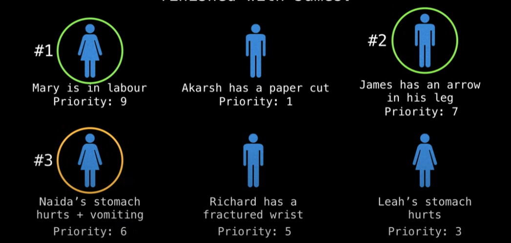
Problems: Hospital Example

Suppose we have people who need to be taken care of, and it really depends on their conditions. For example, Mary is in labor, which has a higher priority than the others. Here is the issue: Richard went to a different hospital, and doesn’t really need to be taken care of anymore, and Nadia’s stomach pain + vomiting turned out to be an infectious disease, so she moved to high priority. This means our priority queue needs to be updated.

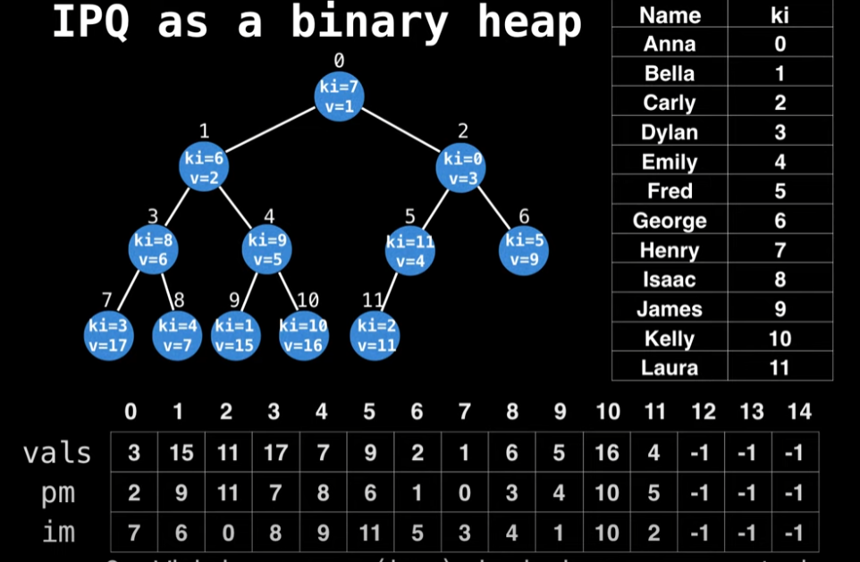
In the hospital example, we saw that it’s crucial to be able to dynamically update the priority (values) of certain people (keys). The Indexed Priority Queue (IPQ) data structure lets us do this efficiently. The first step in using an IPQ is to assign index values to all the keys, forming a bidirectional mapping.

Create a bidriectional mapping between your N keys and the domain [0, N) using a bidrectional hashtable.

Key             |   Key Index
"Marry"        <->    0
"Akarsh"       <->    1
"James"        <->    2
"Naida"        <->    3
"Richard"      <->    4
"Leah"         <->    5

There are several operations in IPQ as following and their time complexity: | Operations | Time Complexity | |——|————| | Empty() | O(1) | | Contains(key) | O(1) | | Size() | O(1) | | Insert() | O(log N) | | MinIndex() - Peek | O(1) | | MinKey() - Peek| O(1) | | DelMin(key) | O(log N) | | KeyOf() & ValueOf(key) | O(1) | | ChangeKey() | O(log N) | | DecreaseKey(key, value) & update | O(log N) | | IncreaseKey(key, value) & update | O(log N) | | Delete() & Update() | O(log N) | | Exch(key, key) | O(1) | | Greater() | O(1) | | Swim(value) | O(log N) | | Sink(value) | O(log N) |

Then why do I metion, it’s bidrectional mapping? Given the key value, we should be able to find the where this node is positioned in heap(position mapping). Also, Given the index value in value table, we should also be able to find the key value.

To show what is bidrectional, look at the image below:

Implementation

template<typename Key>
class IndexMinPQ
{
public:
    IndexMinPQ(int cap)
    {
        capacity = cap;
        size = 0;
        keys.resize(capacity + 1);
        pq.resize(capacity + 1);
        inverseMap.resize(capacity + 1, -1) // InverseMap
    }

    bool Empty()
    {
        return size == 0;
    }

    bool Contains(int i)
    {
        return inverseMap[i] != -1;
    }

    int Size() { return size; }

    void Insert(int i, Key key) 
    {
        size += 1;
        inverseMap[i] = size;
        pq[size] = i;
        keys[i] = key;
        Swim(size);
    }

    int MinIndex()
    {
        return pq[1];
    }

    Key MinKey()
    {
        return keys[pq[1]];
    }

    int DelMin()
    {
        int m = pq[1];
        Exch(1, size--);
        Sink(1);
        inverseMap[m] = -1;
        keys[m] = 0.0;
        pq[size + 1] = -1;
        return m;
    }

    Key keyOf(int i)
    {
        return keys[i];
    }

    void ChangeKey(int i, Key key)
    {
        if (!Contains(i)) {
        	throw::std::invalid_argument("index does not exist");
        }

        if (key < keys[i]) {
        	keys[i] = key;
        	Swim(qp[i]);
        }
        else if (key > keys[i]) {
        	keys[i] = key;
        	Sink(qp[i]);
        }
    }

    void DecreaseKey(int i, Key key)
    {
        keys[i] = key;
        Swim(qp[i]);
    }

    void IncreaseKey(int i, Key key)
    {
        keys[i] = key;
        Swim(inverseMap[i]);
    }

    void Delete(int i)
    {
        int index = inverseMap[i];
        Exch(index, size--);
        Swim(index);
        Sink(index);
        keys[i] = 0.0;
        inverseMap[i] = -1;
    }

    void Exch(int i, int j) // swap
    {
        int swap = pq[i];
        pq[i] = pq[j];
        pq[j] = swap;
        inverseMap[pq[i]] = i;
        inverseMap[pq[j]] = j;
    }

    bool Greater(int i, int j)
    {
        return keys[pq[i]] > keys[pq[j]];
    }

    void Swim(int k)
    {
        while(k > 1 && Greater(pq[k/2], pq[k])){
            Exch(k / 2, k);
            k /= 2;
        }
    }

    void Sink(int k)
    {
        while(2 * k <= size)
        {
            int j = 2 * k;
            if (j < size && Greater(j, j+1))
                j++;
            if (!Greater(k, j)) break;
            Exch(k, j);
            k = j;
        }
    }

private:
    int size = 0;
    int capacity = 0;
    vector<int> pq;
    vector<int> inverseMap;
    vector<Key> keys;
}

The most important operation would be Swim and Sink.

The Swim operation works as follows:

1. Start with the element at index k that needs to be “swum up” the heap
2. Loop until either:
   • We reach the root of the heap (k > 1)
   • The parent is not greater than the current element (!Greater(pq[k/2], pq[k]))
3. In each iteration:
   • Compare the current element with its parent (located at index k/2)
   • If the parent is greater than the current element (in a min heap), exchange them (Exch(k/2, k))
   • Update k to the parent’s position (k /= 2) to continue moving up the heap

Sink Operation needs to go down the heap, which means we need to check both children. Here’s the complete process:

1. Loop until we reach the bottom of the tree (while 2*k <= size)
2. Calculate the index of the left child (j = 2*k)
3. Compare left and right children (if j < size && Greater(j, j+1))
4. If the right child exists (j < size) and is smaller than the left child (Greater(j, j+1)), select the right child by incrementing j
5. This ensures we select the smaller of the two children in a min heap
6. Check if the current node is already smaller than the selected child (!Greater(k, j))
7. If so, the heap property is satisfied, so break out of the loop
8. If not, exchange the current node with the selected child (Exch(k, j))
9. Update k to the position of the child (k = j) and continue the process

Resource

• IndexMinPQ Youtube
• IndexMinPQ

• Reviewing what I studied, how this work will be explained as well.

Dynamic Programming is a method for solving a complex problem by breaking it down into simpler sub-problems. It’s one of a method for solving optimization problems. There are two components of Dynamic Programming:

1. Optimal Substructure
2. Overlapping Subproblems

Optimal Substructure

Optimal Substructure means that the optimal solution to a problem can be constructed from optimal solutions to its sub-problems. Basically, if you break it down to smaller array from big array, and you have an optimal solution to smaller array, you can use it to solve the big array. But when you think about this Optimal Substructure, it’s similar to Divide and Conquer. However there are differences. For example, in Divide and Conquer, we divide the big array into smaller array (divide), calculate, combine, and merge. But we try to find the set of sub-problems that have optimal solutions, and use it to solve the big problem. Also, we can compared this with Greedy Algorithm. Within all the solution that we get from optimal substructure (which is the set of sub-problems), we choose the best solution is the greedy algorithm.

This is normally done by using recursion.

Overlapping Subproblems

When we solve the problem using recursion, we solve the same sub-problem multiple times. This is called Overlapping Subproblems. For example, in the Fibonacci sequence, we can conclude in the following way:

             [ 1 ] n = 1
fib =        [ 1 ] n = 2 
             [ fib(n-1) + fib(n-1) ], n = 3, 4, 5, ...

Then, we can simply draw the tree of the sub-problems (draw yourself!). Then we can see that, fib(4) = fib(3) + fib(2) is calculated twice. This is called Overlapping Subproblems. Then, we can use the same sub-problem as cache to solve the problem.

Two types of Dynamic Programming

• Top-Down (Memoization)
• Bottom-Up (Tabulation)

Top-Down (Memoization)

• Solve the sub-problem using recursing
• Memoize the overlapping sub-problems
• Reuse the memoized sub-problems to solve the big problem

Bottom-Up (Tabulation)

• Solve the sub-problem using iteration
• Using the tabulation, we can store the result of the sub-problem in a table

When to use Dynamic Programming?

• State Transition
• Simple Condition -> Fibonacci, Tiling, Digit DP(if digit condition is met, count the number of cases)
• Array -> Kadane’s algorithm (sub-array sum), Kapsack Problem, Matrix(DAG, #of Path, Path Cost), String(LIS, LCS, Edit Distance), Max Profit (Buy and Sell Stock), Rod Cutting, Matrix Chain Multiplication
• Tree -> DAG, DAG Shortest Path, DAG Longest Path, DAG Topological Sort, # of BST.
• Optimization Problem -> Convex Hull, Matrix Multiplication Order

• Reviewing what I studied, how this work will be explained as well.

Dijkstra Algorithm is a shortest path algorithm that finds the shortest path from a starting node to all other nodes in a graph. Instead of using BFS, it uses priority queue to find the shortest path.

Constraints:

• No negative weight edges
• No negative cycles

This is not dependent on the how many nodes we are passing through, but the weight of the edges. (distance in this case.)

Let’s see the steps of the algorithm.

1. Initialize the distance of the starting node to 0, and the rest of the nodes to infinity.
2. Push the starting node to the priority queue & Pop the starting node from the priority queue.
3. Update the distance of the adjacent nodes (setting infinity to the edge weight), then push them to the priority queue.
4. Then select the node with the smallest distance from the priority queue and repeat the process.

Code is as follows.

#include <iostream>
#include <list>
#include <vector>
#include <limits>
#include <queue>
#include <iomanip>

using namespace std;

// Sedgewick p. 642
class DirectedEdge
{
public:
	int v;         // edge tail
	int w;         // edge head
	double weight; // edge weight

	DirectedEdge(int v, int w, double weight)
	{
		this->v = v;
		this->w = w;
		this->weight = weight;
	}

	double Weight() { return weight; }
	int From() { return v; }
	int To() { return w; }
};

class EdgeWeightedDigraph
{
public:
	int num_vertices;
	int num_edges;
	vector<vector<DirectedEdge>> adj;

	EdgeWeightedDigraph(int num_vertices)
	{
		this->num_vertices = num_vertices;
		this->num_edges = 0;
		adj.resize(this->num_vertices);
	}

	void AddEdge(DirectedEdge e)
	{
		adj[e.From()].push_back(e);
		num_edges += 1;
	}

	vector<DirectedEdge>& Adj(int v) { return adj[v]; }
};

class DijkstraShortestPaths
{
public:
	DijkstraShortestPaths(EdgeWeightedDigraph& g, int s)
		:
		prev(g.num_vertices, -1),
		dist(g.num_vertices, numeric_limits<double>::infinity()),
		visited(g.num_vertices, false)
	{
		dist[s] = 0.0; // distance for self is 0

		pq.push(pair<double, int>{ 0.0, s });

		PrintIndex(dist);
		PrintDist(dist);

		while (!pq.empty())
		{
			int v = pq.top().second;
			pq.pop();

			if (visited[v]) continue;
			visited[v] = true;

			Relax(g, v);
		}

		PrintPaths();
	}

	void Relax(EdgeWeightedDigraph& g, int v)
	{
		// Get the edge of the v
		for (DirectedEdge& e : g.Adj(v)) {
			int w = e.To();
			
			if (visited[w]) continue;

			// update
			double new_dist = dist[v] + e.Weight();
			if (dist[w] > new_dist) {
				dist[w] = new_dist;

				prev[w] = e.From();
				pq.push({ dist[w], w});
			}
		}
		PrintDist(dist);
	}

	void PrintIndex(vector<double>& dist)
	{
		cout << "Vertex: ";
		for (int i = 0; i < dist.size(); i++)
			cout << setw(6) << i;
		cout << endl;
	}

	void PrintDist(vector<double>& dist)
	{
		cout << "Dist  : ";
		for (int i = 0; i < dist.size(); i++)
			cout << setw(6) << dist[i];
		cout << endl;
	}

	void PrintPaths()
	{
		for (int i = 0; i < prev.size(); i++) {
			deque<int> path;
			path.push_front(i);
			int v = prev[i];
			while (v != -1) {
				path.push_front(v);
				v = prev[v];
			}

			for (auto v : path) {
				cout << v;
				if (v != path.back())
					cout << "->";
			}
			cout << endl;
		}
	}

private:
	vector<int> prev;     
	vector<double> dist;
	vector<bool> visited;

	priority_queue<pair<double, int>, vector<pair<double, int>>, greater<pair<double, int>>> pq;
};

The update function is shown below, as new_distance is smaller than the current distance, we update the distance and push the node to the priority queue.

double new_dist = dist[v] + e.Weight();
	if (dist[w] > new_dist) {
		dist[w] = new_dist;

		prev[w] = e.From();
		pq.push({ dist[w], w});
}

Time Complexity

• If we use just a simple array, you can get O(V^2), but if you use priority queue, you can get (V+E) * LogV because priority queue insertion / deletion (Log V), then this happens for each Vertex => V * Log V. Edge Iteration => O(E) Then for relaxation, we update the distance to add that edge would be E * LogV. So we can conclude that it is (V+E) LogV in average. So, sum all it up (O(ELogV + E + VLogV)) => O(V+E logV).

Resource

• C++ Data Structures and Algorithm Design Principles: Leverage the power of modern C++ to build robust and scalable applications

• Reviewing what I studied, how this work will be explained as well.

Binary Heap is a complete binary tree that satisfies the heap property.

Heap Property

• Max-Heap : Parent node is greater than or equal to child node.
• Min-Heap : Parent node is less than or equal to child node.

Heap Constraints

1. Access the max element instantaneously (that’s why the max element in in the root) -> Max Heap

   Min Heap

2. which extends to the idea that, the parent node should be bigger than the children node.
3. Swap (If we are to insert the last element into last tree level, then we need to compare the value, and update the tree)

Heap Operations

• Search (O(N))
• Deletion (Log N)
• Peek (O(1))
• Insertion (Log N) -> Worst Case / But Best Case is O(1)
• Heapify (O(N))

Heapify

If you take a look at the heapify function, it is a function that takes an array, and makes it a heap. So this approximation can be done as follows.

In the logic, we don’t calculate the leaf nodes, we only did siftDown from the first non-leaf node (which is second last node). Maximum number of nodes in each level is floor(n_total / 2^h+1). (h is the height of the tree). Then we can calculate this… 1 * n/4 + 2 * n/8 + 3 * n/16 + … + h * n/2^(h+1).. then n/4 {1 + 2/4 + 3/8 + 4/16 + … + h/2^(h-1)}.. then n/4 {1 + 1/2 + 1/4 + 1/8 + … + 1/2^(h-1)}.. then n/4 {1 / (1 - 1/2)^2} = n. (1/(1-x)^2) = sigma(n *x^(n-1)). This is why it is O(N).

Heap Implementation

struct MaxHeap {
    vector<int> heap;

    MaxHeap() {
        heap.resize(1); // heap 은 무조건 1 부터 시작, 안보이는 0 이 존재
    }

    // ---- priority queue
    void push(int x) {
        int index = int(heap.size());
        heap.push_back(x);
        siftUp(index);
    }

    void siftUp(int index) {
        for (int i = index; i > 1 && heap[i / 2] < heap[i]; i /= 2)  // O(logN)
            swap(heap[i / 2], heap[i]);
    }

    int top() const {
        return heap[1];    
    }

    bool pop() {
        int N = int(heap.size());
        if (N <= 1)
            return false;
        swap(heap[1], heap[N - 1]);
        heap.pop_back();
        siftDown(1);
        return true;
    }

    void siftDown(int index) {
        int N = int(heap.size());
        cout << N << endl;
        for (int i = index, j = index * 2; j < N; i = j, j *= 2) {
            if (j + 1 < N && heap[j] < heap[j + 1])
                j++;
            if (heap[i] >= heap[j])
                break;
            swap(heap[i], heap[j]);
        }
    }

    void heapify(const int arr[], int size) {
        heap.resize(1);
        heap.insert(heap.end(), arr, arr + size);
        
        for (int i = size / 2; i >= 1; i--)
            siftDown(i);
    }
};

The interesting fact about this heap.

Let’s mark that the parent heap is denoted as i, then child on left is i * 2, and right is i * 2 + 1. If you actually draw the tree, parent node is 0001, then left child is 0010, and right child is 0011. then parent node is 0100, left child is 0101, and right child is 0110. then parent node is 0111, left child is 1000, and right child is 1001. then parent node is 1010, left child is 1011, and right child is 1100.

This is interesting! Why? from the parent node, the resulting of left child is shifting left by 1, and right child is shifting left by 1 and adding 1. Then we can back track how many parent nodes are from the child node. For example, if node 9 is 1001, remove MSB, 001. We can see that 0(left)->0(left)->1(right) in that direction, so we have three parent nodes from child node 9.

In the next post, I will show you the leet code problem that uses this heap property.

• LeetCode - Diet Plan Performance

How to Solve

int dietPlanPerformance(vector<int>& calories, int k, int lower, int upper) {
    int points = 0;
    int current_sum = 0;

    for (int i = 0; i < calories.size(); i++) {
        current_sum += calories[i]; // 일단 현재의 Current Sum 을 구한다.

        if (i - k >= 0) {                           // 만약 윈도우 사이즈를 넘어가면, 왼쪽 원소를 빼준다. 즉 이말은 즉슨, k = 1 이면 전에 있던 0 을 빼줘, 1 만 보게끔 하는것이다. 
            current_sum -= calories[i - k]; 
        }

        if (i - k + 1 >= 0) {                      // 윈도우의 시작점 Index 다. k = 2 라고 하면, i - k + 1 = 0 이, 0 부터 만들어진다는 뜻이다. 
            if (current_sum < lower) {
                points--;
            } else if (current_sum > upper) {
                points++;
            }
        }
    }
}

Review

하… Easy 라고 했는데 오랜만에 하니까, Sliding Window 문제가 생각이 안나서 좀 헤맸다. Sliding Windows 라는건 Array[i] 가 있다고 하면, w size 만큼 윈도우를 옮겨가면서 처리하는 문제를 말한다.

Given the root of a complete binary tree, return the number of the nodes in the tree.

According to Wikipedia, every level, except possibly the last, is completely filled in a complete binary tree, and all nodes in the last level are as far left as possible. It can have between 1 and 2h nodes inclusive at the last level h.

Design an algorithm that runs in less than O(n) time complexity.

You can use the priority queue to solve this problem or use the property of the complete binary tree.

class Solution {
public:
    int getHeight(TreeNode* node) {
        int height = 0;
        TreeNode* curr = node;
        while (curr) {
            height++;
            curr = curr->left;
        }
        return height;
    }

    bool exist(TreeNode* root, int index){
        int h = 0;
        for (int i = index; i > 1; i >>= 1)
            h++;
        
        TreeNode* curr = root;
        while(curr) {
            if (h == 0)
                return true;
            if (index & (1 << --h))
                curr = curr->right;
            else 
                curr = curr->left;
        }
        return false;
    }

    int countNodes(TreeNode* root) {
        if (root == nullptr) return 0;

        int h = getHeight(root);
        int lo = 1 << (h - 1); // 8
        int hi = (1 << h) - 1;
        while(lo <= hi){
            int mid = lo + (hi - lo)/2;
            if (!exist(root, mid))
                hi = mid -1;
            else
                lo = mid + 1;
        }
        return hi;
    }
};