Reviewing what I studied, how this work will be explained as well.
Rod Cutting Problem is a problem that we have a rod of length n and we want to cut the rod into n pieces, and we want to maximize the profit. For example, let’s look at the table below. If I have a rod of length 4, then we have 4 ways to cut the rod. Then we calculate the profit for each case
Cut the rod into 1, 1, 1, 1 => max profit = 1 + 1 + 1 + 1 = 4
Cut the rod into 2, 2 => max profit = 5 + 5 = 10
Cut the rod into 3, 1 or 1, 3 => max profit = 8 + 1 = 9
Then, let’s do bottom-up, Bottom-up Apprach is called tabulation, so we need kinda like table. I would say bottom up approch can be more familier if you are good at for-loop! (jk)
But when we think about the time complexity. it would be depending on the O (length). Of course, we do have space complexity which is about O(length + 1).
Reviewing what I studied, how this work will be explained as well.
Index Min Priority Queue
We’ve covered binary heap, priority queue and so forth, but one of the useful priority queue we’re going to look at is Index Min Priority Queue. This is a traditional priority queue variant which on top of the regular PQ operations supports quick updates and deletions of key-value pairs (for example, key can be double type, and value is int type).
Problems: Hospital Example
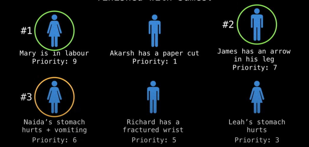
Suppose we have people who need to be taken care of, and it really depends on their conditions. For example, Mary is in labor, which has a higher priority than the others. Here is the issue: Richard went to a different hospital, and doesn’t really need to be taken care of anymore, and Nadia’s stomach pain + vomiting turned out to be an infectious disease, so she moved to high priority. This means our priority queue needs to be updated.
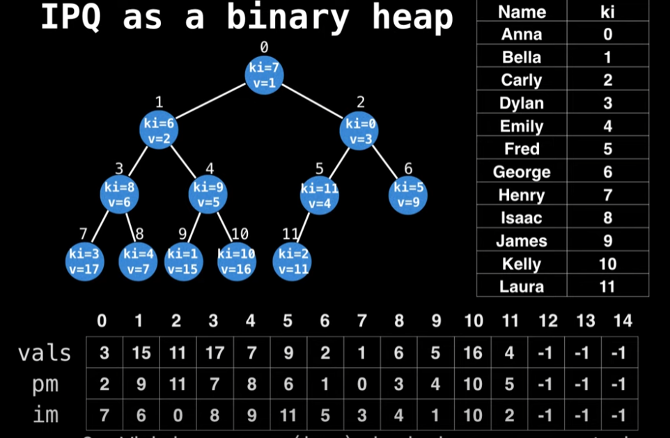
In the hospital example, we saw that it’s crucial to be able to dynamically update the priority (values) of certain people (keys). The Indexed Priority Queue (IPQ) data structure lets us do this efficiently. The first step in using an IPQ is to assign index values to all the keys, forming a bidirectional mapping.
Create a bidriectional mapping between your N keys and the domain [0, N) using a bidrectional hashtable.
Then why do I metion, it’s bidrectional mapping? Given the key value, we should be able to find the where this node is positioned in heap(position mapping). Also, Given the index value in value table, we should also be able to find the key value.
To show what is bidrectional, look at the image below:
Implementation
template<typenameKey>classIndexMinPQ{public:IndexMinPQ(intcap){capacity=cap;size=0;keys.resize(capacity+1);pq.resize(capacity+1);inverseMap.resize(capacity+1,-1)// InverseMap}boolEmpty(){returnsize==0;}boolContains(inti){returninverseMap[i]!=-1;}intSize(){returnsize;}voidInsert(inti,Keykey){size+=1;inverseMap[i]=size;pq[size]=i;keys[i]=key;Swim(size);}intMinIndex(){returnpq[1];}KeyMinKey(){returnkeys[pq[1]];}intDelMin(){intm=pq[1];Exch(1,size--);Sink(1);inverseMap[m]=-1;keys[m]=0.0;pq[size+1]=-1;returnm;}KeykeyOf(inti){returnkeys[i];}voidChangeKey(inti,Keykey){if(!Contains(i)){throw::std::invalid_argument("index does not exist");}if(key<keys[i]){keys[i]=key;Swim(qp[i]);}elseif(key>keys[i]){keys[i]=key;Sink(qp[i]);}}voidDecreaseKey(inti,Keykey){keys[i]=key;Swim(qp[i]);}voidIncreaseKey(inti,Keykey){keys[i]=key;Swim(inverseMap[i]);}voidDelete(inti){intindex=inverseMap[i];Exch(index,size--);Swim(index);Sink(index);keys[i]=0.0;inverseMap[i]=-1;}voidExch(inti,intj)// swap{intswap=pq[i];pq[i]=pq[j];pq[j]=swap;inverseMap[pq[i]]=i;inverseMap[pq[j]]=j;}boolGreater(inti,intj){returnkeys[pq[i]]>keys[pq[j]];}voidSwim(intk){while(k>1&&Greater(pq[k/2],pq[k])){Exch(k/2,k);k/=2;}}voidSink(intk){while(2*k<=size){intj=2*k;if(j<size&&Greater(j,j+1))j++;if(!Greater(k,j))break;Exch(k,j);k=j;}}private:intsize=0;intcapacity=0;vector<int>pq;vector<int>inverseMap;vector<Key>keys;}
The most important operation would be Swim and Sink.
The Swim operation works as follows:
Start with the element at index k that needs to be “swum up” the heap
Loop until either:
We reach the root of the heap (k > 1)
The parent is not greater than the current element (!Greater(pq[k/2], pq[k]))
In each iteration:
Compare the current element with its parent (located at index k/2)
If the parent is greater than the current element (in a min heap), exchange them (Exch(k/2, k))
Update k to the parent’s position (k /= 2) to continue moving up the heap
Sink Operation needs to go down the heap, which means we need to check both children. Here’s the complete process:
Loop until we reach the bottom of the tree (while 2*k <= size)
Calculate the index of the left child (j = 2*k)
Compare left and right children (if j < size && Greater(j, j+1))
If the right child exists (j < size) and is smaller than the left child (Greater(j, j+1)), select the right child by incrementing j
This ensures we select the smaller of the two children in a min heap
Check if the current node is already smaller than the selected child (!Greater(k, j))
If so, the heap property is satisfied, so break out of the loop
If not, exchange the current node with the selected child (Exch(k, j))
Update k to the position of the child (k = j) and continue the process
Reviewing what I studied, how this work will be explained as well.
Dynamic Programming is a method for solving a complex problem by breaking it down into simpler sub-problems. It’s one of a method for solving optimization problems. There are two components of Dynamic Programming:
Optimal Substructure
Overlapping Subproblems
Optimal Substructure
Optimal Substructure means that the optimal solution to a problem can be constructed from optimal solutions to its sub-problems. Basically, if you break it down to smaller array from big array, and you have an optimal solution to smaller array, you can use it to solve the big array. But when you think about this Optimal Substructure, it’s similar to Divide and Conquer. However there are differences. For example, in Divide and Conquer, we divide the big array into smaller array (divide), calculate, combine, and merge. But we try to find the set of sub-problems that have optimal solutions, and use it to solve the big problem. Also, we can compared this with Greedy Algorithm. Within all the solution that we get from optimal substructure (which is the set of sub-problems), we choose the best solution is the greedy algorithm.
This is normally done by using recursion.
Overlapping Subproblems
When we solve the problem using recursion, we solve the same sub-problem multiple times. This is called Overlapping Subproblems. For example, in the Fibonacci sequence, we can conclude in the following way:
             [ 1 ] n = 1
fib =        [ 1 ] n = 2
             [ fib(n-1) + fib(n-1) ], n = 3, 4, 5, ...
Then, we can simply draw the tree of the sub-problems (draw yourself!). Then we can see that, fib(4) = fib(3) + fib(2) is calculated twice. This is called Overlapping Subproblems. Then, we can use the same sub-problem as cache to solve the problem.
Two types of Dynamic Programming
Top-Down (Memoization)
Bottom-Up (Tabulation)
Top-Down (Memoization)
Solve the sub-problem using recursing
Memoize the overlapping sub-problems
Reuse the memoized sub-problems to solve the big problem
Bottom-Up (Tabulation)
Solve the sub-problem using iteration
Using the tabulation, we can store the result of the sub-problem in a table
When to use Dynamic Programming?
State Transition
Simple Condition -> Fibonacci, Tiling, Digit DP(if digit condition is met, count the number of cases)
Array -> Kadane’s algorithm (sub-array sum), Kapsack Problem, Matrix(DAG, #of Path, Path Cost), String(LIS, LCS, Edit Distance), Max Profit (Buy and Sell Stock), Rod Cutting, Matrix Chain Multiplication
Tree -> DAG, DAG Shortest Path, DAG Longest Path, DAG Topological Sort, # of BST.
Optimization Problem -> Convex Hull, Matrix Multiplication Order
Reviewing what I studied, how this work will be explained as well.
Dijkstra Algorithm is a shortest path algorithm that finds the shortest path from a starting node to all other nodes in a graph. Instead of using BFS, it uses priority queue to find the shortest path.
Constraints:
No negative weight edges
No negative cycles
This is not dependent on the how many nodes we are passing through, but the weight of the edges. (distance in this case.)
Let’s see the steps of the algorithm.
Initialize the distance of the starting node to 0, and the rest of the nodes to infinity.
Push the starting node to the priority queue & Pop the starting node from the priority queue.
Update the distance of the adjacent nodes (setting infinity to the edge weight), then push them to the priority queue.
Then select the node with the smallest distance from the priority queue and repeat the process.
Code is as follows.
#include<iostream>
#include<list>
#include<vector>
#include<limits>
#include<queue>
#include<iomanip>usingnamespacestd;// Sedgewick p. 642classDirectedEdge{public:intv;// edge tailintw;// edge headdoubleweight;// edge weightDirectedEdge(intv,intw,doubleweight){this->v=v;this->w=w;this->weight=weight;}doubleWeight(){returnweight;}intFrom(){returnv;}intTo(){returnw;}};classEdgeWeightedDigraph{public:intnum_vertices;intnum_edges;vector<vector<DirectedEdge>>adj;EdgeWeightedDigraph(intnum_vertices){this->num_vertices=num_vertices;this->num_edges=0;adj.resize(this->num_vertices);}voidAddEdge(DirectedEdgee){adj[e.From()].push_back(e);num_edges+=1;}vector<DirectedEdge>&Adj(intv){returnadj[v];}};classDijkstraShortestPaths{public:DijkstraShortestPaths(EdgeWeightedDigraph&g,ints):prev(g.num_vertices,-1),dist(g.num_vertices,numeric_limits<double>::infinity()),visited(g.num_vertices,false){dist[s]=0.0;// distance for self is 0pq.push(pair<double,int>{0.0,s});PrintIndex(dist);PrintDist(dist);while(!pq.empty()){intv=pq.top().second;pq.pop();if(visited[v])continue;visited[v]=true;Relax(g,v);}PrintPaths();}voidRelax(EdgeWeightedDigraph&g,intv){// Get the edge of the vfor(DirectedEdge&e:g.Adj(v)){intw=e.To();if(visited[w])continue;// updatedoublenew_dist=dist[v]+e.Weight();if(dist[w]>new_dist){dist[w]=new_dist;prev[w]=e.From();pq.push({dist[w],w});}}PrintDist(dist);}voidPrintIndex(vector<double>&dist){cout<<"Vertex: ";for(inti=0;i<dist.size();i++)cout<<setw(6)<<i;cout<<endl;}voidPrintDist(vector<double>&dist){cout<<"Dist : ";for(inti=0;i<dist.size();i++)cout<<setw(6)<<dist[i];cout<<endl;}voidPrintPaths(){for(inti=0;i<prev.size();i++){deque<int>path;path.push_front(i);intv=prev[i];while(v!=-1){path.push_front(v);v=prev[v];}for(autov:path){cout<<v;if(v!=path.back())cout<<"->";}cout<<endl;}}private:vector<int>prev;vector<double>dist;vector<bool>visited;priority_queue<pair<double,int>,vector<pair<double,int>>,greater<pair<double,int>>>pq;};
The update function is shown below, as new_distance is smaller than the current distance, we update the distance and push the node to the priority queue.
If we use just a simple array, you can get O(V^2), but if you use priority queue, you can get (V+E) * LogV because priority queue insertion / deletion (Log V), then this happens for each Vertex => V * Log V. Edge Iteration => O(E) Then for relaxation, we update the distance to add that edge would be E * LogV. So we can conclude that it is (V+E) LogV in average. So, sum all it up (O(ELogV + E + VLogV)) => O(V+E logV).
Reviewing what I studied, how this work will be explained as well.
Binary Heap is a complete binary tree that satisfies the heap property.
Heap Property
Max-Heap : Parent node is greater than or equal to child node.
Min-Heap : Parent node is less than or equal to child node.
Heap Constraints
Access the max element instantaneously (that’s why the max element in in the root) -> Max Heap
Min Heap
which extends to the idea that, the parent node should be bigger than the children node.
Swap (If we are to insert the last element into last tree level, then we need to compare the value, and update the tree)
Heap Operations
Search (O(N))
Deletion (Log N)
Peek (O(1))
Insertion (Log N) -> Worst Case / But Best Case is O(1)
Heapify (O(N))
Heapify
If you take a look at the heapify function, it is a function that takes an array, and makes it a heap. So this approximation can be done as follows.
In the logic, we don’t calculate the leaf nodes, we only did siftDown from the first non-leaf node (which is second last node). Maximum number of nodes in each level is floor(n_total / 2^h+1). (h is the height of the tree). Then we can calculate this… 1 * n/4 + 2 * n/8 + 3 * n/16 + … + h * n/2^(h+1).. then n/4 {1 + 2/4 + 3/8 + 4/16 + … + h/2^(h-1)}.. then n/4 {1 + 1/2 + 1/4 + 1/8 + … + 1/2^(h-1)}.. then n/4 {1 / (1 - 1/2)^2} = n. (1/(1-x)^2) = sigma(n *x^(n-1)). This is why it is O(N).
Heap Implementation
structMaxHeap{vector<int>heap;MaxHeap(){heap.resize(1);// heap 은 무조건 1 부터 시작, 안보이는 0 이 존재}// ---- priority queuevoidpush(intx){intindex=int(heap.size());heap.push_back(x);siftUp(index);}voidsiftUp(intindex){for(inti=index;i>1&&heap[i/2]<heap[i];i/=2)// O(logN)swap(heap[i/2],heap[i]);}inttop()const{returnheap[1];}boolpop(){intN=int(heap.size());if(N<=1)returnfalse;swap(heap[1],heap[N-1]);heap.pop_back();siftDown(1);returntrue;}voidsiftDown(intindex){intN=int(heap.size());cout<<N<<endl;for(inti=index,j=index*2;j<N;i=j,j*=2){if(j+1<N&&heap[j]<heap[j+1])j++;if(heap[i]>=heap[j])break;swap(heap[i],heap[j]);}}voidheapify(constintarr[],intsize){heap.resize(1);heap.insert(heap.end(),arr,arr+size);for(inti=size/2;i>=1;i--)siftDown(i);}};
The interesting fact about this heap.
Let’s mark that the parent heap is denoted as i, then child on left is i * 2, and right is i * 2 + 1. If you actually draw the tree, parent node is 0001, then left child is 0010, and right child is 0011. then parent node is 0100, left child is 0101, and right child is 0110. then parent node is 0111, left child is 1000, and right child is 1001. then parent node is 1010, left child is 1011, and right child is 1100.
This is interesting! Why? from the parent node, the resulting of left child is shifting left by 1, and right child is shifting left by 1 and adding 1. Then we can back track how many parent nodes are from the child node. For example, if node 9 is 1001, remove MSB, 001. We can see that 0(left)->0(left)->1(right) in that direction, so we have three parent nodes from child node 9.
In the next post, I will show you the leet code problem that uses this heap property.
intdietPlanPerformance(vector<int>&calories,intk,intlower,intupper){intpoints=0;intcurrent_sum=0;for(inti=0;i<calories.size();i++){current_sum+=calories[i];// 일단 현재의 Current Sum 을 구한다.if(i-k>=0){// 만약 윈도우 사이즈를 넘어가면, 왼쪽 원소를 빼준다. 즉 이말은 즉슨, k = 1 이면 전에 있던 0 을 빼줘, 1 만 보게끔 하는것이다. current_sum-=calories[i-k];}if(i-k+1>=0){// 윈도우의 시작점 Index 다. k = 2 라고 하면, i - k + 1 = 0 이, 0 부터 만들어진다는 뜻이다. if(current_sum<lower){points--;}elseif(current_sum>upper){points++;}}}}
Review
하… Easy 라고 했는데 오랜만에 하니까, Sliding Window 문제가 생각이 안나서 좀 헤맸다. Sliding Windows 라는건 Array[i] 가 있다고 하면, w size 만큼 윈도우를 옮겨가면서 처리하는 문제를 말한다.
Given the root of a complete binary tree, return the number of the nodes in the tree.
According to Wikipedia, every level, except possibly the last, is completely filled in a complete binary tree, and all nodes in the last level are as far left as possible. It can have between 1 and 2h nodes inclusive at the last level h.
Design an algorithm that runs in less than O(n) time complexity.
You can use the priority queue to solve this problem or use the property of the complete binary tree.
Unreal Object 가 만들어지기 위해서는, 실제 컴파일 전에 Unreal Header Tool 에 헤더 파일 분석하는 과정에서 선행이 되며, 이 과정이 완료되면, Intermediate Folder 에 Unreal Object 정보를 담음 Meta File 이 생성 된다.
이 Meta 정보는 Unreal Engine이 지정한 UClass 라는, 특별한 클래스를 통해서 보관됩니다.
UClass 에는 Unreal Object 에 대한 클래스 계층 구조 정보와 멤버 변수, 함수에 대한 정보를 모두 기록하고 있습니다.
하지만 단순히 검색하는 것에서 더 나아가, Run Time 에서 특정 클래스를 검색해 형(Type) 을 알아내 인스턴스의 멤버 변수 값을 변경하거나 특정 인스턴스의 member function 호출하는것이 가능하다.
Reflection
Java / C# 과 같은 경우 Reflection 이라는 이름으로 제공
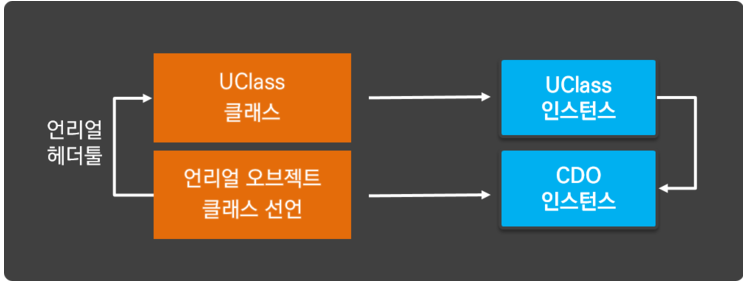
Compile 단계에서 Unreal Object 마다 UCLass 가 생성된다면, 실행 초기의 Run Time 과정에서는 Unreal Object 마다 Class 의 정보와 함께 Unreal Object 의 Instance 가 생성됩니다.
이 특별한 Instance 는 Unreal Object 의 기본 세팅을 지정하는데 사용되는데, 이를 클래스 기본 객체 (Class Default Object: CDO) 라고 한다.
Unreal Engine 에서 CDO 를 만드는 이유는 Unreal Object 를 생성할 떄마다 매번 초기화를 시키지 않고, 기본 인스턴스를 미리 만들어 놓고 복제하는 방식으로 메커니즘이 구성되어 있기 때문이다.
예를 들어서 복잡한 기능을 수행하는 캐릭터를 담당하고, 기능이 커진다고 했을때 굉장히 큰덩어리로 될수 있다. 이럴때 100 개의 instance 를 만든다고 가정하면, 캐릭터를 하나씩 처음부터 생성 하고, 초기화 시키는 방법보다, 미리 큰 기본 객체 덩어리를 복제하고, 속성 값만 변경하는게 더 효율적이기 때문이다.
정리하자면, 아래와 같이 하나의 Unreal Object 가 초기화 될 때에는 두개의 Instance 가 항상 생성 됩니다.
이 생성자 클래스는 Instance 를 초기화 해 CDO 를 제작하기 위해서 사용되고, 초기화에서만 실행되고, 실제 게임 플레이에서는 생성자 코드를 사용할 일이 없다.
Unreal Engine 에서 게임 플레이에서 사용할 초기화 함수는 생성자 대신 Init() 이나 혹은 BeginPlay() 함수를 제공
위의 코드는 cardianl 이라는 std::vector<int> 타입이 존재 했을때, const_iterator type 으로 begin 과 end 를 각각 iter 와 iter_end 로 변수로 지정해놓았다. 그리고 while 문 에서는 total element 에다가 vector 에 있는 모든 int 을 곱해서 결국은, 벡터의 모든 원소들의 곱을 나타낸다.
이런 방법도 있지만, 조금 더 Modern C++ 로 다른 방법으로 해결한다면 Functor 를 이용할수 있다.
하지만 위의 코드는 product 라는 struct 를 만들고, for_each 로 while 문을 대신해서 사용된다. 하지만 struct 에 대한 operator 그리고 constructor 를 지정하므로 코드가 생각보다 길어진다. 그렇다면 어떻게 더 간단하게 만들수 있을까? 아래의 코드를 보자. 아래의 코드가 바로 lambda 로 구성한 코드이다.
각각의 부분은 introducer(capture), parameters, return type, statement 로 구성이 되어있다. introducer 같은 경우는 [] 안에 있는 my_mod 라는 변수를 람다 내부에서 사용할 수 있게 된다. 그리고, parameter: () 안에서는, 받을 인자를 적게 되는데 위의 예에서는 int 형을 가지고 와서 lambda 내부에서 사용할 수 있게 된다. trailing_return type 같은 경우는 따로 말하지는 않겠다. 이런 한 lambda 식을 결국은 쓰게된다. 여기서 바로 closure 과 lambda expression 에서 이야기를 하게 된다.
lambda expression 을 쓰긴 하지만, Runtime 에는 이름이 없지만, 메모리 상에 임시적으로 존재하는 Closure 가 생성이된다. 예를 들어보자. 아래의 = 옆에 부분에 lambda expression 이 있다고 가정하면, 결국 Runtime 에 closure 가 생성이되고, f 는 closure 에 대한 복사값이 될것이다. 물론 closure 를 복사하는 부분은 std::move 로 넘길수 있지만 f 가 closure 는 아니다.
autof=[&](intx,inty){returnfudgeFactor*(x+y);};
실제 closure object 는 이 statement 가 끝났을때, 파괴된다. 즉 closure 과 lambda 의 차이는 정확하게 클래스와 클래스 인스턴스의 차이인거다. 결국 class 같은 경우는 정의를 한거고, closure 는 class 의 instance 이다. 결국 class 는 소스코드에만 존재하고, runtime 에서는 존재 하지않고, class instance 들은 run time 에 존재하게 되는것들이다.