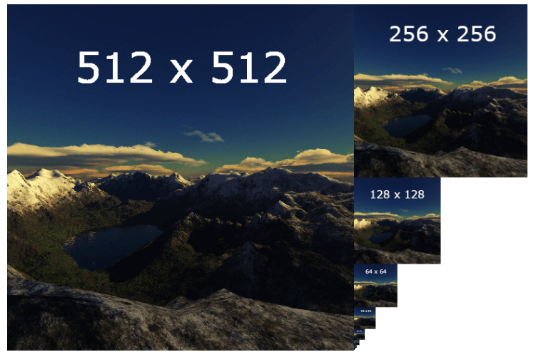
Mipmap 이라는건 Main Texture Image 를 downsized 를 시킨 여러개의 사진이라고 생각하면 된다. 즉 여러개의 해상도를 조정하며 만든 여러개의 Image 라고 생각 하면 된다. Computer Vision 에서는 Image Pyramid 라고도 하는데, 여러개의 서로 다른 Resolution 의 Image 를 올려 놓았다고 볼수 있다. 아래의 이미지를 봐보자. 아래의 Image 를 보면 512, 512/2, 256/2… 절반씩 Resolution 이 줄어들고 있다.
그러면 어디서 이게 사용되까? 라고 한다면 바로 MIPMAP 이다. MIPMAP vs Regular Texture 라고 하면, 바로 문제가 Aliasing 이 문제이다. 아래의 Image 를 보면 이해할수 있을것 같다.
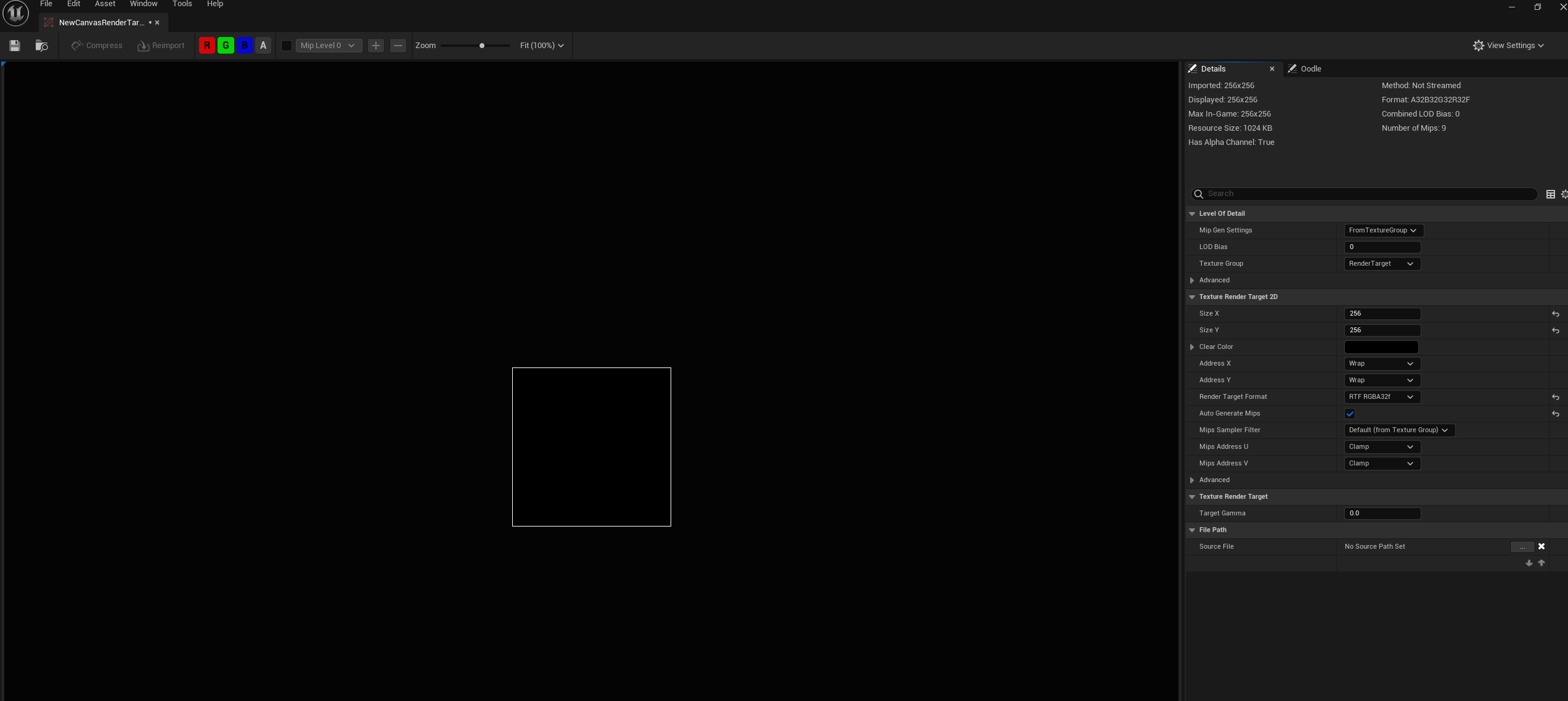
Unreal 에도 똑같은 기능이 있는데, 바로 RenderTargetTexture 를 생성시에 여러가지의 옵션이 보인다.
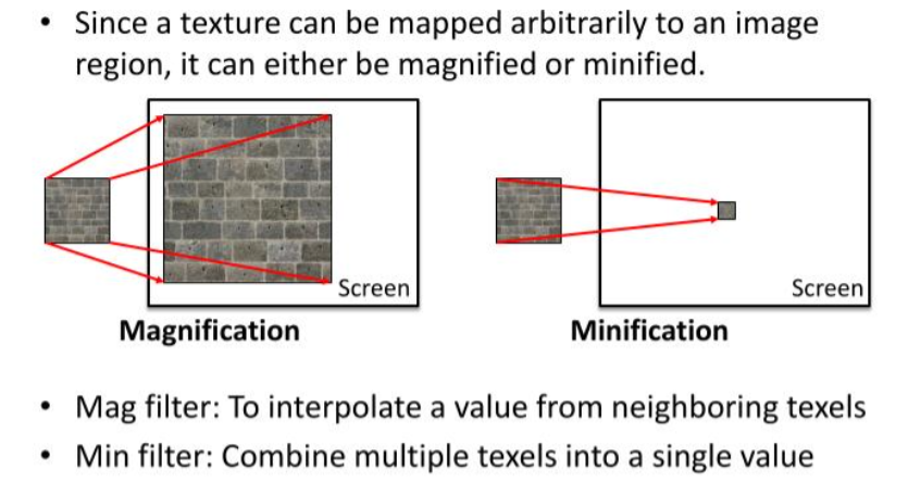
옵션을 보면, Texture RenderTarget 2D 라고 해서, DirectX 에서 사용하는 description 을 생성할때와 동일한 옵션이 된다. 여기에서 Mips Filter(Point Sampler / Linear Interpolation Sampler) 도 보인다. 결국에는 Texture 를 Mapping 한다는 관점에서, 우리는 Texture Coordinate 을 어떠한 사각형 박스 안에 Mapping 을 해서 사용했고, 그걸 사용할때, Texture Coordinate 도 명시를 했었다. 자 결국에는 Texture 를 Mapping 한다는 관점에서 봤을때, 확대도 가능하고, 축소도 가능하다. 그게 바로 Maginification 과 Minification 이다.
즉 Magnification 을 하기 위해서, Mag Filter (To interpolate a value from neihboring texel) 이말은 결국엔 Linear Filter / Pointer Filter 로 Interpolation 과 그리고 내가 그리려는 Texture (64, 64) 를 어떠한 박스 (512, 512) 에 붙인다고 상상했을때, 그림은 작고, 보여줘야하는 화면이 클경우, GPU 가 이 Texture 를 늘려서 보간을 해야하는 경우가 (그말은 화면 하나의 픽셀이 원래 텍스쳐의 중간쯤 위치에 거릴수 있다. texel / pixel < 1) Magnification 이라고 한다. 그리고 이 반대의 상황을 Minification 이라고 한다. 그리고 MipLevels = 0 으로 둔다는게 Max MipMap 즉 MipMap 을 Resolution 대로 만들고 이게 결국에는 LOD 와 똑같게된다.
Subresoruce Term 인데, Texture 의 배열로 각각 다른 Texture 에 대해서, 각각의 Mipmap 들을 생성한는것이 바로 Array Slice 이고, 여러개의 Texture 에서. 같은 Resolution 끼리, mipmap level 이 같은걸 MIP Slice 라고 한다. A Single Subresoruce(Texture) 즉 하나의 Resource 안에서, Subresource 를 선택해서 골라갈수 있다. (이걸 Selecting a single resource) 라고 한다. 자세한건, Subresource 를 확인하면 좋다.
아래의 코드를 보자면 추가된건 별로 없지만, Staging Texture 임시로 데이터를 놓는다. 그 이유는 MipMap 을 생성할때, 우리가 내부의 메모리가 어떻게 되어있는지 모르므로, 최대한 안전하게 Input Image 를 StagingTexture 를 만들어 놓고, 그리고 실제로 사용할 Texture 를 설정을 해준다. 이때 Staging 한거에대해서 복사를 진행하기에, D3D11_USAGE_DEFAULT 로 설정을 하고, 그리고 GPU 에게 결국에는 RESOURCE 로 사용할것이다 라는걸 Description 에 넣어주고, Mip Map 을 설정한다. (즉 GPU 에서 GPU 에서 복사가 이루어진다.) 즉 Staging Texture는 GPU 리소스에 직접 데이터를 쓸 수 없기 때문에, CPU 쓰기 전용 텍스처에 데이터를 쓴 후 GPU용 리소스로 복사하는 중간 단계라고 말을 할수 있겠다. 그리고 메모리만 잡아놓고, CopySubresourceRegion 을 통해서, StagingTexture 를 복사를 한다. 그리고 마지막에 그 해당 ResourceView 에, 이제 GenerateMips 를 하면 될것 같다.
CPU
ComPtr<ID3D11Texture2D>texture;ComPtr<ID3D11ShaderResourceView>textureResourceView;ComPtr<ID3D11Texture2D>CreateStagingTexture(ComPtr<ID3D11Device>&device,ComPtr<ID3D11DeviceContext>&context,constintwidth,constintheight,conststd::vector<uint8_t>&image,constintmipLevels=1,constintarraySize=1){D3D11_TEXTURE2D_DESCtxtDesc;ZeroMemory(&txtDesc,sizeof(txtDesc));txtDesc.Width=width;txtDesc.Height=height;txtDesc.MipLevels=mipLevels;txtDesc.ArraySize=arraySize;txtDesc.Format=DXGI_FORMAT_R8G8B8A8_UNORM;txtDesc.SampleDesc.Count=1;txtDesc.Usage=D3D11_USAGE_STAGING;txtDesc.CPUAccessFlags=D3D11_CPU_ACCESS_WRITE|D3D11_CPU_ACCESS_READ;ComPtr<ID3D11Texture2D>stagingTexture;HRESULThr=device->CreateTexture2D(&txtDesc,nullptr,stagingTexture.GetAddressOf())if(FAILED(hr)){cout<<"Failed to Create Texture "<<endl;}D3D11_MAPPED_SUBRESOURCEms;context->Map(stagingTexture.Get(),NULL,D3D11_MAP_WRITE,NULL,&ms);uint8_t*pData=(uint8_t*)ms.pData;for(UINTh=0;h<UINT(height);h++){memcpy(&pData[h*ms.RowPitch],&image[h*width*4],width*sizeof(uint8_t)*4);}context->Unmap(stagingTexture.Get(),NULL);returnstagingTexture;}ComPtr<ID3D11Texture2D>stagingTexture=CreateStagingTexture(device,context,width,height,image);D3D11_TEXTURE2D_DESCtxtDesc;ZeroMemory(&txtDesc,sizeof(txtDesc));txtDesc.Width=width;txtDesc.Height=height;txtDesc.MipLevels=0;// Highest LOD LeveltxtDesc.ArraySize=1;txtDesc.Format=DXGI_FORMAT_R8G8B8A8_UNORM;txtDesc.SampleDesc.Count=1;txtDesc.Usage=D3D11_USAGE_DEFAULT;txtDesc.BindFlags=D3D11_BIND_SHADER_RESOURCE|D3D11_BIND_RENDER_TARGET;txtDesc.MiscFlags=D3D11_RESOURCE_MISC_GENERATE_MIPS;txtDesc.CPUAccessFlags=0;// Copy the highest resolution from the staging texturecontext->CopySubresourceRegion(texture.Get(),0,0,0,0,stagingTexture.Get(),0,nullptr);// Creating Resource Viewdevice->CreateShaderResourceView(texture.Get(),0,textureResourceView.GetAddressOf());// Generate Mipmap reducing the resolutioncontext->GenerateMips(textureResourceView.Get());
GPU 에서는 결국에는 Mipmap 을 사용해줘야하므로, HLSL 에서는 그냥 Sample() 아니라 SampleLevel() 을 해줘야한다. 참고로 Sample() 과 SampleLevel 의 차이는 Sample 을 이용하면, lod Level 을 내부적으로 계산해서 샘플링을 한다고 한다. 그리고 LOD 가 0 이면 Quality 가 좋은 Texture 라고 정할수 있다. (Vertex 개수가 많음).
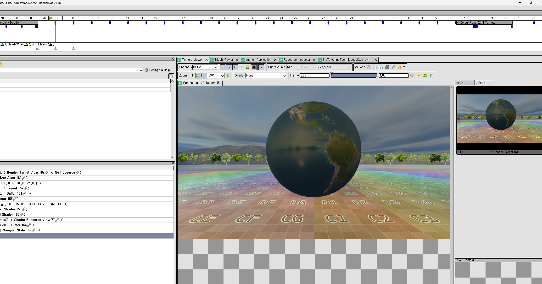
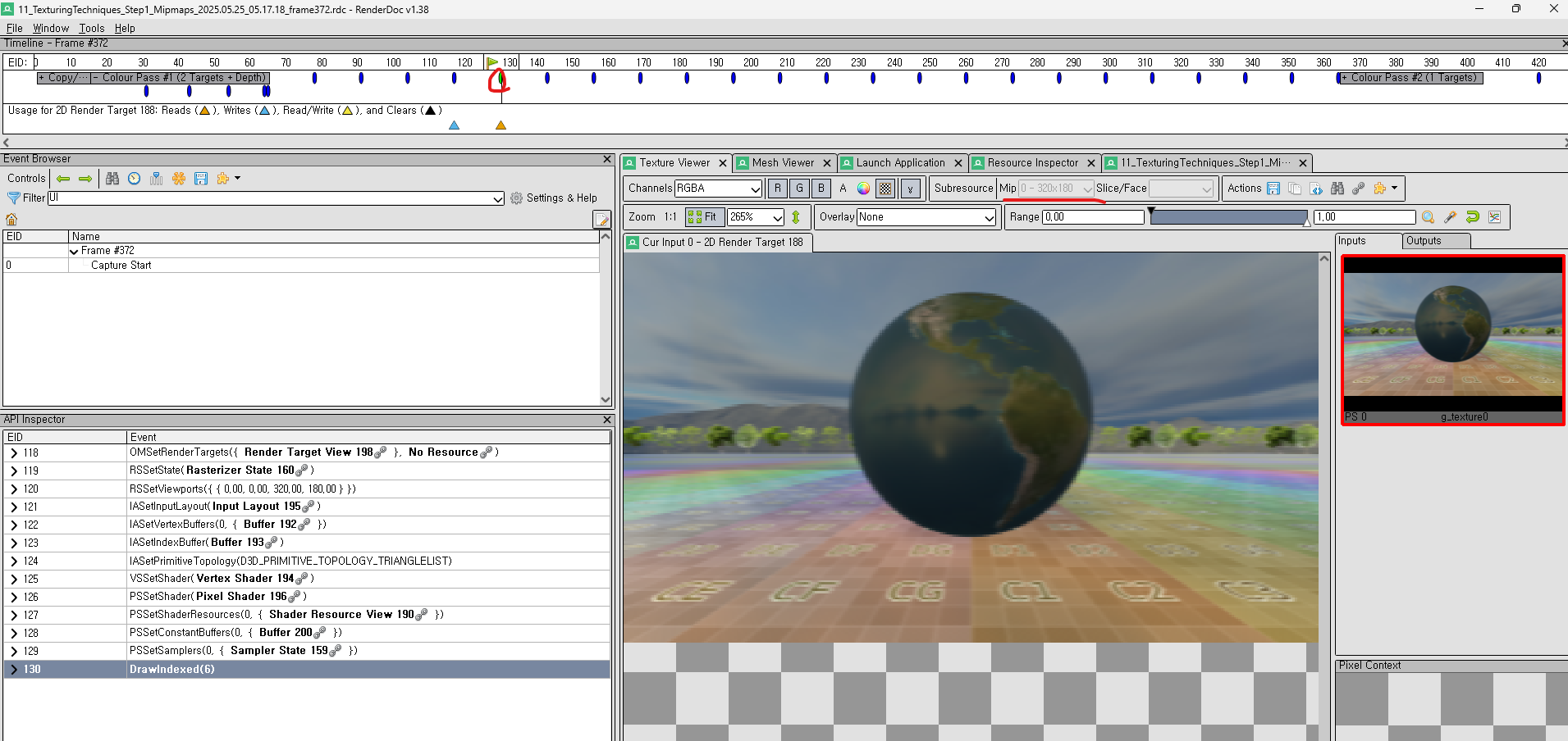
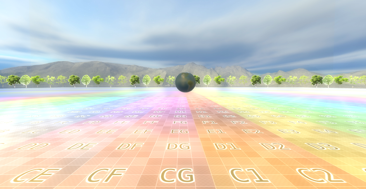
또, 이렇게 끝내면 좋지 않지 않느냐? 바로 RenderDoc 으로 부터 언제 MipMap 이 생성되는지 한번 봐야하지 않겠냐 싶어서 RenderDoc 을 돌려봤다. PostPorcessing 이 끄면 이 MipMap 들이 보이진 않을거다. 즉 한 Pass 와 다른 Pass 사이에 MipMap 을 내부적으로? 생성하는것 같아보인다. 제일 앞에 있는게 제일 높은 LOD 를 가지고 있다. 그리고 RenderDoc 에서 왜 클릭이 안되어있는지는 모르겠지만 Subresource 를 보면 Mip Level 들이 보이고, 내부적으로 해상도(Size) 를 계속 줄이는것 같이 보인다.
2024 년 6 월 3 일 부터 시작된 독일 출장 및 ADAS Testing Expo 전시회를 갔다. 솔직히 말하면, 출장 가는데 너무 준비할 서류도 많고, 여러가지로 오해도 많았어서, 하나하나 하는데 조금 힘겨웠었다. 물론 이런저런걸 따지기에는 에너지 소비가 많이됬다. 그리고 전시회를 가는 인원들이 전부다 high level 사람들이라서 교류하는것도 굉장히 힘들거라는 생각을 먼저 하다보니, 이것 저것으로 고민이 많았다. 하지만 결론적으로 말하면 그 무엇보다도 독일 사람들의 기본적인 성향과 Testing Expo 에서 우리 회사가 정말로 필요한게 무엇이 있는지와 내가 정말 좋아하는게 뭔지를 더욱더 잘알수 있게 되는 계기가 되지 않았을까 생각이 들었다.
물론 나는 이걸로 하여금, Simulation 이 되게 양날의 검이라는걸 너무 깨닫게 되었다. 물론 Simulation Environment 에서 할 수 있는 것들이 많지만, 그래도 한계가 분명 존재 할것이다. 특히나 상용 엔진을 계속 사용한다면과 우리 회사에서 하고 있는 여러 Project 들이 한 Product 에 녹아 들지 않으면, 이건 결국엔 잡다한 기능을 다가지고 있는 Simulator 라는 기능밖에 되지 않는다라는걸 알게 되었다. 이게 좋은 Career 이 될지는 굉장히 많은 의심이 되고, 하지만 결국엔 좋은 Product 를 가꾸기 위해서는 각 분야의 최고의 사람들과 일을 할수 있는 기회가 분명 필요하겠다라는 생각이 아주 많이 들었다. 특히나 한국 회사의 특성상 “이거 해줘! 기능은 일단 알아서 해줘봐 피드백 줄께” 이런식이 되버려서 참 어렵다는건 정말 알겠다. 하지만 이러한 방식으로 Hardware 의 Product 가 나온다고 했을때 분명 고장나고 사람들에 입맛에 맞지 않아서 결국엔 버려질 운명이다라는 생각밖에 안든다. 분명 Software Engineering 관점에서는 어떠한 Pipeline 이 구성되지 않은 상황속 및 Senior Engineer 가 없다고 한다면, 정말 Junior 들이 시간을 많이 투자하고, 공부하는데 정말 많은 Resource 가 필요할거다! 라는 생각 밖에 들지 않았다.
긍정적으로 봤을때는, 다른 회사와 경쟁할수 있다는 점과, 그리고 다른 회사 사람들의 의견이나 앞으로의 가능성 이런걸 판단했을때, 옳은 시장성을 가지고 있다는건 분명하다. 어떠한 분야에 몰입있기에는 정말 수많은 시간과 노력이 필요하다! 라는건 정말 뼈저리게 느껴버렸던 출장 이였다.
어쩌다보니 Logging System 을 만들고, 기록은 해놓아야 할 것 같아서, Singleton 패턴에 대해서 c++ 로 정리 하려고 한다. Singleton 이라는건 Class 를 딱 하나만 생성한다 라고 정의한다라는게 정의된다. static 으로 정의를 내릴수 있다. 그리고 객체가 복사가 이루어지면 안된다. 일단 싱글톤을 만든다고 하면, 하나의 설계 패턴이므로 나머지에 영향이 안가게끔 코드를 짜야된다. 일단 Meyer’s implementation 을 한번 봐보자.
classSingleton{public:staticSingleton&getInstance();{staticSingletoninstance;returninstance;}private:Singleton(){}// no one else can create one~Singleton(){}// prevent accidental deletion// disable copy / move Singleton(Singletonconst&)=delete;Signleton(Singleton&&)=delete;Singleton&operator=(Singletonconst&)=delete;Singleton&operator=(Singleton&&)=delete};
그렇다면 더확실하게 생성과 파괴의 주기를 확실하게 보기위해서는 아래와 같이 사용할수 있다.
classSingleton{public:staticstd::shared_ptr<Singleton>getInstance();{staticstd::shared_ptr<Signleton>s{newSingleton};returns;}private:Singleton(){}// no one else can create one~Singleton(){}// prevent accidental deletion// disable copy / move Singleton(Singletonconst&)=delete;Signleton(Singleton&&)=delete;Singleton&operator=(Singletonconst&)=delete;Singleton&operator=(Singleton&&)=delete};
예제를 들어보자, 뭔가 기능상으로는 Random Number Generator 라고 하자. 아래와 같이 구현을 하면 좋을 같다.
classRandom{public:staticRandom&Get(){staticRandominstance;returninstance;}staticfloatFloat(){returnGet().IFloat();}private:Random(){}~Random();Random(constRandom&)=delete;voidoperator=(Randomconst&)=delete;Random&operator=()floatIFloat(){returnm_RandomGenerator;}// internalfloatm_RandomGenerator=0.5f;};intmain(){// auto& instance = Singleton::Get(); // this is good practice// Single instance = Singleton::Get(); // Copy this into new instance; Just want a single instance.floatnumber=Random::Get().Float();return0;}
You are given an array prices where prices[i] is the price of a given stock on the ith day. You want to maximize your profit by choosing a single day to buy one stock and choosing a different day in the future to sell that stock. Return the maximum profit you can achieve from this transaction. If you cannot achieve any profit, return 0.1
Implementation
This is typical greey probelm, you select one, and compare it to get the maximum or the best output for goal once. This case, you want to maximize the profit, which in this case, you select one prices, and loop through to get the meximum prices.
You are climbing a staircase. It takes n steps to reach the top. Each time you can either climb 1 or 2 steps. In how many distinct ways can you climb to the top?
Approach
This is typically done in recursive fashion. But think of this. if i have steps 1, 2, 3, … i - 2, i - 1, i. Then, we need to use a step for i - 1 or i - 2 to get to i. This means I have several different steps to get to i. (this satisfies the optimal substructure). we can make a simple S(1) = 1, S(2) = 2, S(n) = S(n - 1) + S(n - 2).
First Implementation:
When I tested this on recursive way and submit, it exceed Time Limit!… Oh no…
Now, I need to use dynamic programming, for top-down approach, it exceed Memory Limit, which possibly because of recursive way of saving into cache won’t work very well.
Given an integer array arr and a 2D integer array queries, where each element of queries represents a query in the form of [s, e, k], perform the following operation for each query: For each query, find the smallest element in arr[i] that is greater than k for all i such that s ≤ i ≤ e. Return an array containing the answers for each query in the order they were processed. If no such element exists for a query, store -1 for that query.
Constraints:
The length of arr is between 1 and 1,000 (inclusive). Each element of arr is between 0 and 1,000,000 (inclusive). The length of queries is between 1 and 1,000 (inclusive). For each query [s, e, k], s and e are between 0 and the length of arr minus 1 (inclusive).
Since, we’re looping through the queries n, which is O(n), but there is inner loop which is start time to end time. In the worst case, it can be O(n^2).
Given an integer array arr and a 2D integer array queries, where each element of queries represents a query in the form of [s, e], perform the following operation for each query: For each query, increment arr[i] by 1 for all i such that s ≤ i ≤ e. Return the array arr after processing all queries according to the above rule.
Constraints:
The length of arr is between 1 and 1,000 (inclusive). Each element of arr is between 0 and 1,000,000 (inclusive). The length of queries is between 1 and 1,000 (inclusive). For each query [s, e], s and e are between 0 and the length of arr minus 1 (inclusive).
Given an integer array nums, return an array answer such that answer[i] is equal to the product of all the elements of nums except nums[i]. The product of any prefix or suffix of nums is guaranteed to fit in a 32-bit integer. You must write an algorithm that runs in O(n) time and without using the division operation.
The major constraint is to calculate the product of array except itself. If you implement in brute force way, you will get O(n^2). However, this is the constraints! We need to solve this problem for O(n) time complexity with no extra space complexity.
Approach
This 2D structure represents the products of all numbers except the one at each index. The second and third lines show how we can calculate the left and right parts separately.
24,2,3,41,12,3,41,2,8,41,2,3,6
For the input array , the output array represents the prefix products, which are the products of all numbers to the left of each index. This prefix product is calculated by accumulating the numbers to the left at each iteration.
For instance, in the first iteration, there are no numbers to the left, so it’s just 1. In the second iteration, you have 1 to the left, so the output is 1 * 1 = 1. In the third iteration, you have 1 and 2 to the left, so the output becomes 1 * 2 = 2`, and so on.
This process continues until you have the prefix products for all indices. After calculating the prefix products, you can calculate the suffix products and multiply them with the prefix products to get the final result.
Then you do the right, which are going to be the product of suffix. You can do the same thing from right to left.
Let’s think about this way, we are going to all the power to the sort(), which means the time complexity depends on sort algorithm. Then we can divide three cases:
If the first digit is missing, which is mostly likely 0 if the vector is sorted
If the last digit is missing, which is mostly likely the max Value of the vector.
If the any middle index are missing, starting from 0 to N-1, find the missing number and return the index.
classSolution{public:intmissingNumber(vector<int>&nums){sort(nums.begin(),nums.end());intn=nums.size();if(nums[0]!=0)return0;// 0 is missingif(nums[n-1]!=n)returnn;// if the last character is missingfor(inti=1;i<nums.size();i++){if(nums[i]!=i){returni;}}return0;}};
You are given two non-empty linked lists representing two non-negative integers. The digits are stored in reverse order, and each of their nodes contains a single digit. Add the two numbers and return the sum as a linked list.
You may assume the two numbers do not contain any leading zero, except the number 0 itself.