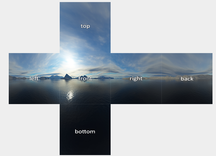
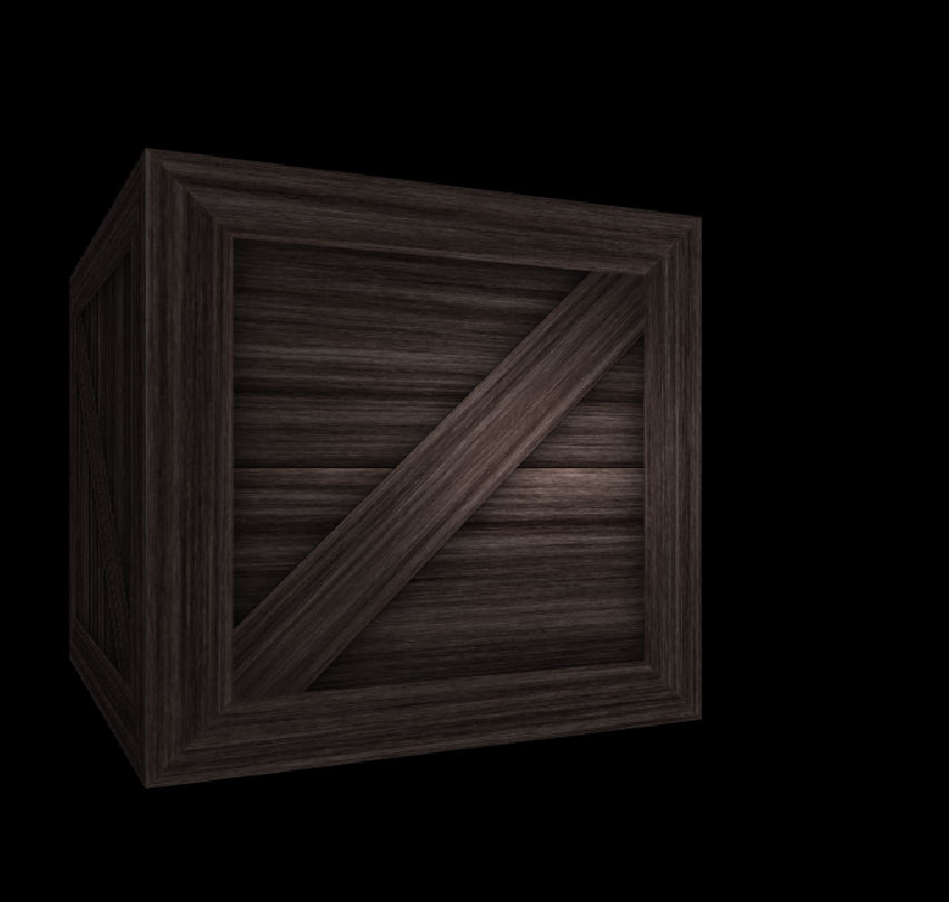
환경적 요소를 다루기 위한 한걸음인것 같다. Cube Mapping 이란건 쉽게 말해서 카메라가 거대한 상자 안에 있는것과 같다. 즉 아래의 그림처럼, 거대한상자는 십자가 패턴으로, 총 6 개의 Textures 로 이루어져있다. 일반 Texture 와 다른 부분이 하나 있다. 전에 같은 경우는 Texture 를 입힌다라고 했을때 Mesh 에다가 Texture 좌표계를 입혔어야했다. Cube Mapping 같은 경우에는 DirectX 내부에서 알아서 해준다고 볼수 있다.
그러면 DirectX 에서 어떻게 Cube Mapping 을 하는지 해보자.
CPU Side
autoskyBox=L"./CubemapTextures/skybox.dds"ComPtr<ID3D11ShaderResourceView>cubemapResourceView;ComPtr<ID3D11Texture2D>texture;HRESULThr=CreateDDSTextureFromFileEx(m_device.Get(),filename,0,D3D11_USAGE_DEFAULT,D3D11_BIND_SHADER_RESOURCE,0,D3D11_RESOURCE_MISC_TEXTURECUBE,DDS_LOADER_FLAGS(false),(ID3D11Resource**)texture.GetAddressOf(),cubemapResourceView.GetAddressOf(),nullptr);if(FAILED(hr)){std::cout<<"Failed To Create DDSTexture "<<std::endl;}// -----// ConstantBufferBasicVertexConstantBuffer{Matrixmodel;MatrixinverseTranspose;Matrixview;Matrixprojection;};static_assert((sizeof(BasicVertexConstantBuffer)%16)==0,"Constant Buffer size must be 16-byte aligned");std::shared_ptr<Mesh>cubeMesh;cubMesh=std::make_shared<Mesh>();BasicVertexConstantBufferm_BasicVertexConstantBufferData;m_BasicVertexConstantBufferData.model=Matrix();m_BasicVertexConstantBufferData.view=Matrix();m_BasicVertexConstantBufferData.projection=Matrix();ComPtr<ID3D11Buffer>vertexConstantBuffer;// This is custom MethodCreateConstantBuffer(m_BasicVertexConstantBufferData,cubeMesh->vertexConstantBuffer);MeshDatacubeMeshData=MeshGenerator::MakeBox(20.0f);std::reverse(cubeMeshData.indicies.begin(),cubeMeshData.indicies.end());CreateVertexBuffer(cubeMeshData.vertices,cubeMesh->vertexBuffer);CreateIndexBuffer(cubeMeshData.indices,cubeMesh->indexBuffer);ComPtr<ID3D11InputLayout>inputLayout;ComPtr<ID3D11VertexShader>vertexShader;ComPtr<ID3D11PixelShader>pixelShader;vector<D3D11_INPUT_ELEMENT_DESC>basicInputElements={{"POSITION",0,DXGI_FORMAT_R32G32B32_FLOAT,0,0,D3D11_INPUT_PER_VERTEX_DATA,0},};CreateVertexShaderAndInputLayout(L"CubeMappingVertexShader.hlsl",basicInputElements,vertexShader,inputLayout);CreatePixelShader(L"CubeMappingPixelShader.hlsl",pixelShader);// Render omit: But this is just update the constant buffer.// Update: Pipeline for cube mappingm_context->IASetInputLayout(inputLayout.Get());m_context->IASetVertexBuffer(0,1,cubeMesh->vertexBuffer.GetAddressOf(),&stride,&offset);m_context->IASetIndexBuffer(cubeMesh->indexBuffer.Get(),DXGI_FORMAT_R32_UINT,0);m_context->IASetPrimitiveTopology(D3D11_PRIMITIVE_TOPOLOGY_TRIANGLELIST);m_context->VSSetShader(vertexShader.Get(),0,0);m_context->VSSetConstantBuffers(0,1,cubeMesh->vertexConstantBuffer.GetAddressOf());ID3D11ShaderResourceView*views[1]={cubemapResourceView.Get()};m_context->PSSetShaderResources(0,1,views);m_context->PSSetShader(pixelShader.Get(),0,0);m_context->PSSetSamplers(0,1,m_samplerState.GetAddressOf());// Start Drawingm_context->DrawIndexed(cubeMesh->m_indexCount,0,0);
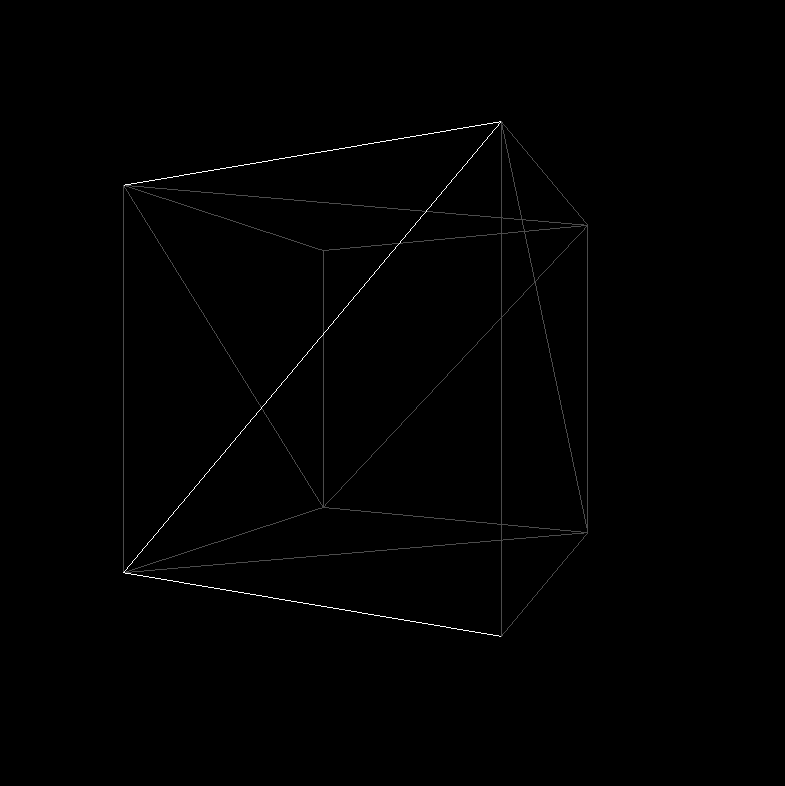
CubeMap Mesh 를 불러온다. (이때 Cubemap 은 Box Mexh, 단 주의점은 너무 크다보면, Camera 시점에서, Far Point 의 조정이 필요하다.)
그 이후에는 CubeMap Texture 를 불러온다. 위의 십자가 모형을 만든 Format (.dds) 를 불러온다.
참고로 dds 는 DirectX 에서 한 Image 의 Format 인데, 주로 Graphics 용도로 사용한다고 한다.
Cubemapping 을 하기위해서는, Shader 가 따로 필요하다 (VertexShader & PixelShader). 그리고 기존에 사용하던 Constant Buffer 도, 일단 수정하지말고 그대로 불러오는 작업을 한다.
Important: CubeMap 같은 경우 카메라가 큐브맵 안에 있으니, 큐브맵이 BackFace 를 바라보는건데, 큐브맵이 Front Face 로 돌려줘야한다. 그러기위해선 기존에, 정점 CCW 로 되어있는게 Front Face 이므로, BackFace(CW) 에 있었던 정점정보들을 CCW 려 돌려줘야한다. (조그만더 정리하자면, 원래 카메라에서 물체를 바라볼때, DirectX 에서는 CCW 로 정점이 생성되서, FrontFace 라고 확인이 되지만 뒤로 봤을때는 이게 CW 로 되어있다. 그래서 Culling 이라는게 존재하는것이다.) 또 다른 방법은 D3D11_CULL_MODE::D3D11_CULL_NONE 을 하면된다.
BackFace 에서 FrontFace 로 변경이후, vertex 와 index 의 정보를 Buffer 에다가 넣어준다.
새로운 Shader 에서 정의를 하니, InputLayout 도 정의를 하고, VertexShader 와 PixelShader 를 생성해준다.
Render 부분에서는 ConstantBuffer Model 의 Position 만 Update 해주는 방식으로 해주는 대신에, 빈 Matrix 를 넣어줘야한다. 왜냐하면 카메라 시점이 바꾼더라도, Mesh Model 은 변경이 안되어야하므로…
그리고 Update 하는 부분쪽이서는 모든 Resources 들을 Shader 에서 볼수 있도록 Binding 을 해준다.
Vertex Shader 에서는 output 에 pos 를 직접 넣어주고, 그리고 Pixel Shader 에서는 Sampling 만 하면 된다.
결과는 아래와 같다.
이러다보면 이상한 점이 있기는한데, 그게 Texture 의 고화질이라고 하면, 사실상 Texture 에 있는 빛처럼 보이는 Source 도 있기 때문에 실제로 어디에 Light Source 가 있는지를 모른다. 그리고, Light Source 로 인해서, Model 의 색깔이나, Shadowing 이런게 잘 보이질 않는다 이걸 해결할수 있는 기법 중에 하나가 Environment Mapping 이다.
DirectX11 - Environment Mapping
결국에는 mapping 을 잘된 결과를 가지고 오기위해서는 Texture 의 Quality 가 좋아야, 그만큼의 조명이 돋보이고, 더 사실적인 Rendering 이 비춰질수 있을것 같다는 생각이든다. 그렇다면 어떻게 하는게 좋을까? 다시 생각을 해보자. 모델이 있다고 하면, 내가 바라보는 시점으로 부터 Model 의 Normal 을 타고 들어간다고 하고, 반사되었을때의 CubeMap 의 Texture 의 값을 가지고 오면 될것 같고, 바라보는 방향과 상관없는것들은 CubeMap 의 Texture 를 그대로 가지고 오면될것 같다.
그러면 변화해야할것들은 무엇인가? 하면, 바로 CubeMap 의 ResourceView 를 넘겨주면 될것 같다. 그러면 다시 CPU 쪽에서 작업을 해주자. 그말은 즉슨 Model 에 우리가 그리는 정보를 줘야하니. Model 에다가 CubeMap 이 그려진 ResourceView 를 Binding 해주면 된다는 의미이다. 그러면 기존의 Pixel Shader 에가 TextureCube 를 넣어주면 된다.
// When Render is Called.// 1. Drawing the CubeMapping on cubmapResourceView// 2. For each Mesh, you set pixel shader for binding two resesources.ID3D11ShaderResourceView*resViews[2]={mesh->textureResourceView.Get(),cubemapResourceView.Get()};m_context->PSSetShaderResources(0,2,resViews);// Updating the constant buffer is omitted for simplicity// Then on GPUTexture2Dg_texture0:register(t0);// Texture on ModelTextureCubeg_textureCube0:register(t1);// Cubemap TextureSamplerStateg_sampler:register(s0);// Sampler StatestructPixelShaderInput{float4posProj:SV_POSITION;// Screen positionfloat3posWorld:POSITION;float3normalWorld:NORMAL;float2texcoord:TEXCOORD;float3color:COLOR;};cbufferBasicPixelConstantBuffer:register(b0){float3eyeWorld;booldummy1;Materialmaterial;Lightlight[MAX_LIGHT];float3rimColor;float3rimPower;float3rimStrength;booldummy2;}float4main(PixelShaderInputinput):SV_TARGET{float3toEye=normalize(eyeWorld-input.posWorld);// Lighting ... returng_textureCube0.Sample(g_sampler,reflect(-toEye,input.normalWorld));}
위의 방식대로 Sample 을 많이 다루다 보면, Sample 의 두번째 Parameter 는 Location 이다. 즉 GPU 에게 Texture 의 어느 위치를 Sampling 할건지를 물어보는거다. 그리고 reflect(…) 같은 경우는 toEye 가 결국에는 Camera 에서 Model 로 향하는 벡터라고 하면, Incident Vector 로 바꿔줘야한다(-toEye) 그리고 Model 의 Normal 을 World 좌표계에서 보여지는걸 넣어주면, 결국엔 그 반사된 Vector 로 부터 Sampling 을 할수 있다는것 이다.
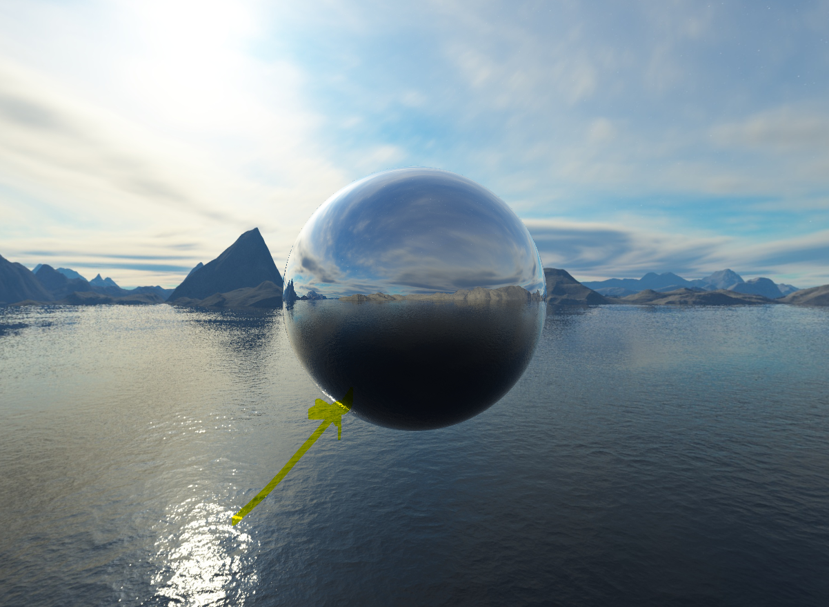
결과는 아래와 같다. 아래 Cubemap 에 위치해있는, 빛의 일부분이 그대로 반사되서 구에 맺히는걸 볼수 있다. 굉장히 아름다운 Graphics 인것 같다.
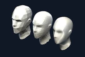
처음으로, Model Import 코드를 짜보고 테스트를 해보았아. Library 는 Assimp 로 3D Model 을 Load 를 하면 된다. 일단 기본적으로 Modeling 에 앞서서 Blender 를 확인 해보자.
이러한식으로 Blender 에서, Model 을 Import 할때 여러가지의 Formats 이 보인다. 내가 다뤄봤던건 아래와같다.
Standford Rabit (.ply) => Point Cloud Data 옮길때
glTF 2.0 (.glb/.gltf) => 이건 기억이 잘안나지만, 이게 최신인걸로 알고 있다.
Wavefront (.obj) => 이건 정말 많이 다뤄본것 같다. (차량 Model, Radar Model, etc..)
일단 3D Modeling Import 는 Assimp Library 로 충분하다. 각 모델을 확인해보면 각 Format 별로 Vertex, Index, Normal 값들이 존재하며, 또 Parts 별 Texture 가 존재한다. 가끔씩은 Normal 값이 존재 안할수도 있는데, 이건 따로 처리해야할필요가 있다. 그리고 확실히 std::fileSystem c++17 부터 나와서 훨씬 Path 정리하는게 편하다.
코드는 StackOverflow 나 GameDev 에서 작성하였다.
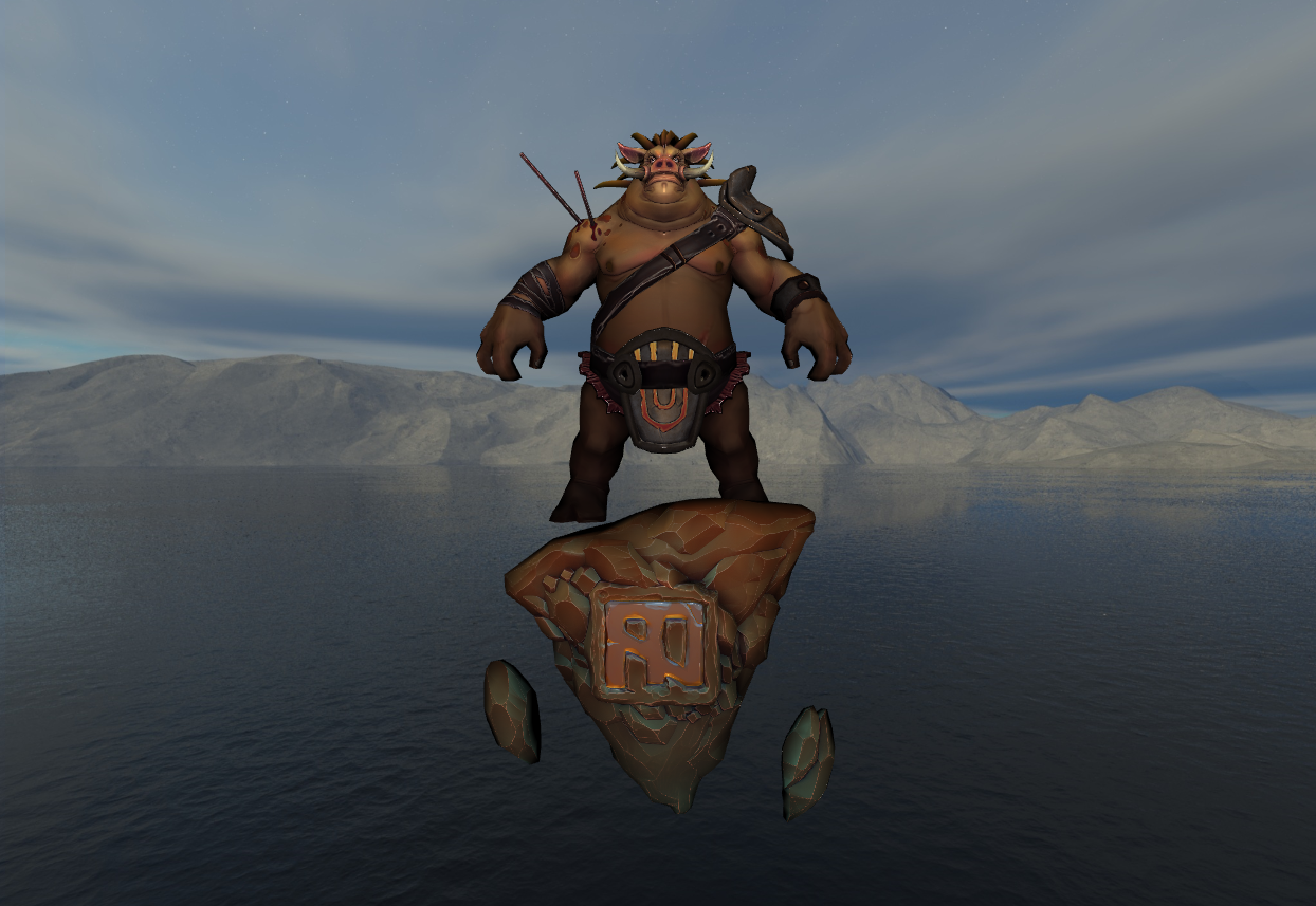
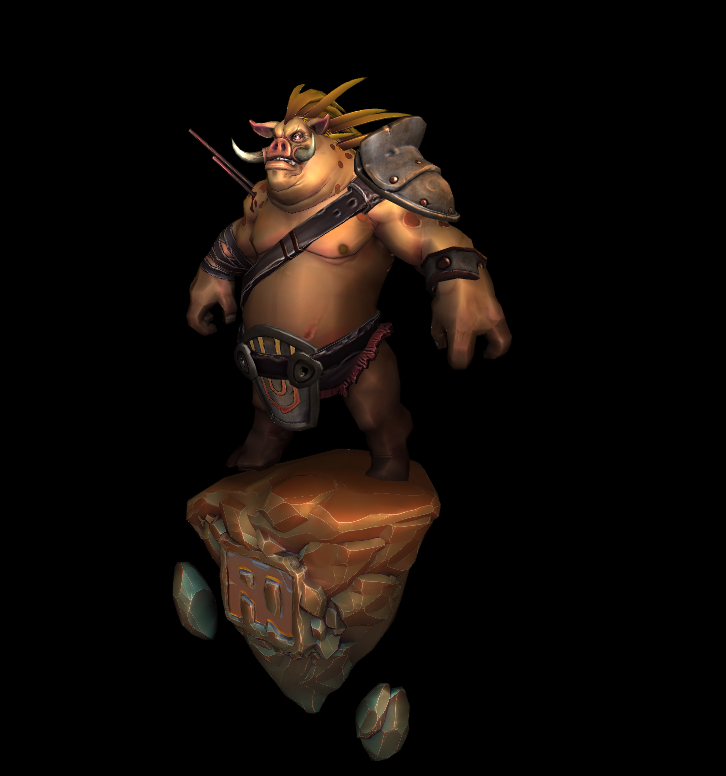
결과를 한번 보자면 아래와 같다. 이런저런 Free Model 이 있는데, sketchFab, glTF, CesiumGS, and f3d 이렇게 있다.
나는 어렸을때, Dota 를 좋아해서, 진짜 Dota Character 인지는 모르겠지만, F3D 에서 Dota 캐릭터를 가지고 왔다. 충분히 Animation 도 있는것 같은데, 아직 Animation 의 구현은 멀어서,,, 일단 Import 된것 까지 한번 봐보자.
이제는 조금은 재밌는 장난을 더해서, Lighting 을 개선해보는게 좋을것 같다. Rim Effect 는 물체의 가장자리 (Edge) 에 빛이 강조되어 반사되는 효과를 뜻한다. 주로 역광 (Backlighting) 상황에서 발생하여, 물체의 윤곽을 강조한다. 즉, 빛이 물체를 직접 비추지 않아도 가장자리에서 빛이 새어 나오는 현상을 뜻한다.
사용되는 용도를 조금 찾아보니, 캐릭터의 윤곽을 강조하거나, 뭔가 환상적인 분위기를 연출하거나, Material 을 표현 할때, 투명하거나 빛을 산란시키는 재질의 특성을 표현한 것이다.
그렇다면 Edge 를 찾으려면 어떻게 해야하는걸까? 일단 생각을 해보면, Model 의 Normal Vector 와 카메라 시점에서 바라본 Vector 의 Normal 값이 90 도가 됬을때, Edge 라고 판별을 할 수 있을것같다. 이제 HLSL 에 적용을 해보자.
이미 이제껏 VertexShader 에 넣어준 ConstantBuffer 의 느낌은 Model, InverseTranspose, view, projection 이 있다. 그리고 각각의 Shader 에서 main 함수의 Parameter 같은 경우는, 아래와 같다.
항상 조심해야 하는건, ConstantBuffer 는 16 의 배수여야한다! 그리고 Specular 를 계산을 할때, pow() 라는걸 사용했었다. 그걸 적절하게 사용을하고, 1.0 - dot(input.normalWorld, toEye) 를 하는데에 있어서는, 각도의 90 도 일때, dot product 값은 0 이다. 이걸 확대하게하기 위해서, 1 을 빼주는것이다. 다른 방법으로는 Saturate 대신에, smoothstep 을 사용해도 괜찮은 결과가 나오는것 같았다.
앞에 Post 를 봤더라면, 이제 Sphere 는 cylinder 의 맨위와 아래의 radius 를 묶으면 되지 않느나라는 질문을 할수 있다. 맞다! 그리고 Stakc 이 총 6개라면, 6 개만큼을 아래서부터 각도를 줘서 구처럼 구부리면 될수 있다.
그러면 수식으로 세우면 이렇다, Vector 의 위치 (0, -radius, 0) 부터 시작해서, Z 축 으로 해서 높이를 쌓고, y 축으로 Vertex 를 돌리면 된다. 그말은 첫 Vertex Point 로 부터 Phi 각도를 점차 점차 올라가면서, Transform 을 해주면 된다. 그래서 간단하게 SimpleMath 를 사용한다면 아래의 코드처럼만 변경하고, Indices 와 Normal 은 Cylinder 와 마찬가지로 하면 된다.
// loop in stacksconstflaotdTheta=-XM_PI/float(numSlices);constfloatdPhi=-XM_PI/float(numStacks);Vector3startPoint=Vector3::Transform(Vector3(0.0,-radius,0.0),Matrix::CreateRotationZ(dPhi*i));// loop in slice// from x-z plane, rotateVertexv;v.position=Vector3::Transform(stackPoint,Matrix::CreateRotationY(dTheta*float(j)));
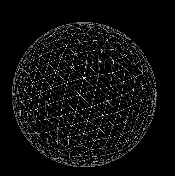
Subdivision
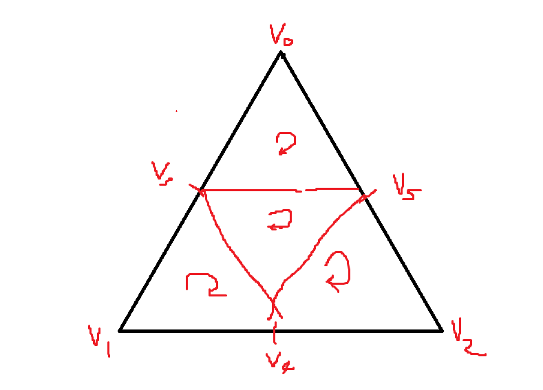
Subdivision 은 여러 방법이 있을텐데, 제일 기본적인 방법은 Triangle Mesh 를 4 개 만들어주는거다. 즉 Vertex Point 들을 부풀려서 준다고 생각을 하면된다. 근데 굳이? 왜 CPU 단에서 부풀리려고 하냐? 굳이 이렇게 만들 필요가 있냐? 라고 하면, Subdivision 같은 경우는 GPU 에서도 충분히 돌릴수 있다. 그래서 아래의 그림을 보면 모형의 조금더 부드럽게 더 늘려서, 물체의 형태를 실제와 같이 Vertex 를 늘려주는 역활이라고 할수 있다.
앞서 말했다 싶이, 제일 기본적인 아이디어는 아래와 같다. 하나의 Triangle Mesh 가 있다고 하면, Vertex 와 Vertex 사이에 중간의 Vertex 를 둬서 다시 연결해줘서 삼각형을 1개에서 4개로 증가 시켜주는 알고리즘이라고 볼수 있다. 그래서 알고리즘은 이렇다. 만약 기존의 Mesh Data 의 Normal 값을 radius 와 곱한다. 즉 vertex position 을 다시 구의 표면위에 작업하는 작업이라고 볼수 있다.
그리고 이러한 방식이 필요한데, 이건 Subdivison 을 할때마다, Texture 들의 좌표가 깨질수도 있으니, 이음매를 엮어주는 형식이다. 그리고 새로운 Mesh Data 에 순서대로 넣어준다고 하고, Indices 들도 정하면, 아래처럼 여러개의 Step 을 돌렸을때 구형이 더 구형처럼 보이게 될것이다.
사실상 Vertex 를 기준으로해서 즉 하나의 각을 기준으로 해서도 우리는 다른 Normal 을 가진다고 생각을 할수 있다. 즉 각 Vertex 별 Face Normal 이 다르다는 말이다. 이건 구현의 그림으로 보면 편할것 같다. 그리고 삼각형에서 결국에는 Face Normal 을 구하는건 하나의 Vector 에서 다른 하나의 Vector 의 Cross Product 한 결과 값이다.
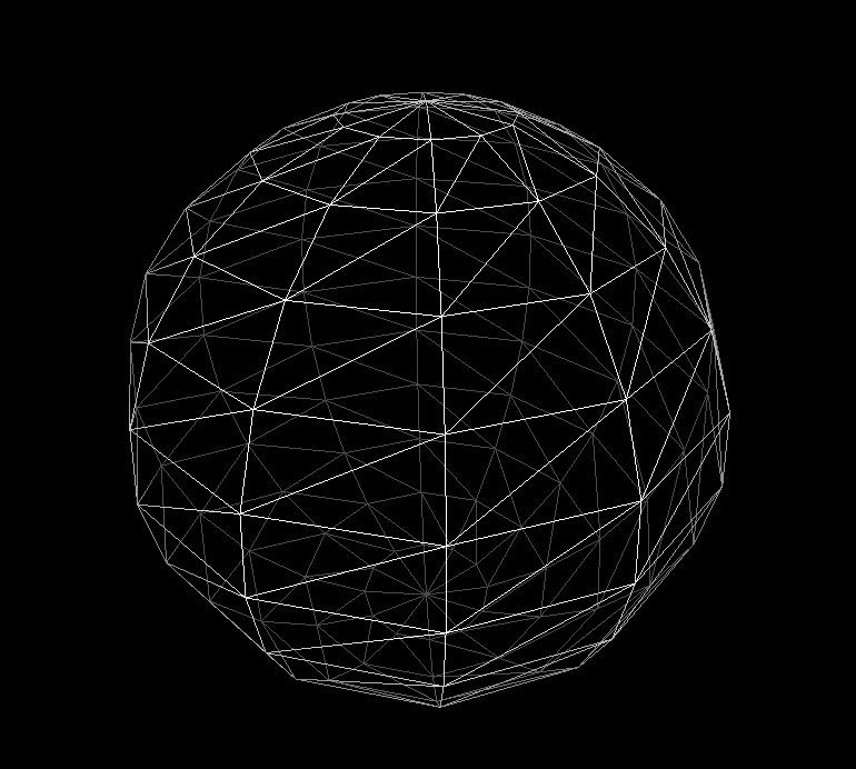
아마 전에 Sphere Modeling 을 Post 를 봤다고 한다면, 약간의 더러움이 보였을거다. 그게 뭔말이냐면… 삼각형이 균일하게 만들어지지 않았다는 점이다. 그리고 아무리 저번처럼 Texture Mapping 에 필요한 공식을 썻더라고 한더란들, 문제는 해결되지 않는다.
일단 그림 부터 한번 참고를 해보는게 좋을것 같다. 일단 최악의 상황일때, 즉 Subdivision 을 안했을때를 한번 봐보자. 이상태에서 보면 저렇게 끊겨져 있는걸 볼수 있을거다. 그 이유중에 하나는, 바로 Texture 의 삼각형안에서 Interpolation 을 하려고 보니 생기는 이슈이다.
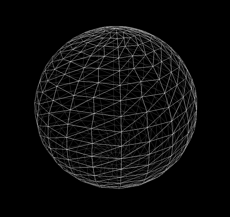
그래서 다시 Subdivision 을 해서 일단 완벽한 구형의 모델을 만들어보자. Wireframe 을 볼수 있다. 아래처럼 일정하게 삼각형들을 그리게 된다고 하면, 아래처럼 똑같이 나온다.
이거에 대한 원인은 Cylinder 를 조금 다시 돌아보면 좋을것 같다. Subdivision 을 했을시에 결과값이 Texture 좌표계에서 0 과 1 로 딱떨어지는 경우에는 잘 Mapping 이 될거다. 하지만, 만약에 Texture 좌표에 애매하게 들어가있더라고 하면 0 과 1 사이를 Interpolation 을 시켜버려서, 저렇게 Pixel 값이 흐트러지는 현상이 나온다. 그래서 해결방법은 그렇다. Texture Coordinate 를 Vertex 단위로 Mapping 하는게 아니라, Pixel 단위로 넘기게 된다면 해결이 될문제이다. 즉 다시 uv 값을 계산해서 Pixel Shader 에서 그리게 하면 된다. uv 값을 계산하는식은 전 Post 에 있으니 그 코드를 Shader 코드로 넘기면 된다.
그걸 해결하기위해서는 이제 Shader Programming 으로 들어가는거다. 이제까지 PixelShader 에서 받는 Input 같은 경우에, projection, world, normalworld, texcoord, color 값을 Parameter 로 CPU 에서 GPU 쪽으로 넘기고 있었다. 이때 model 에 대해서 position 값을 같이 넘겨주면 일단 첫번째 Step 이다. 그리고 Pixel Shader 에서 계산을 할때, uv 를 다시 계산해서, 아래처럼 Sampler 을 시키면 해결이 된다.
이제껏, WireFrame 과 Normal 을 봤다. 또한 중요한 부분중에 하나는 Model 이 우리가 봤던 박스처럼 모든 모델이 그렇게 생겨있지 않다. 예를 들어서 구, Cylinder 등의 모형들은 격자 무늬로 이루어져 있으며, 특히나 지형 같은 경우도 Grid Plane 이라고 볼수 있다. 그럼 Grid Plane 은 어떻게 생겨 먹은 친구 인지 한번 봐보자. 아래를 보면, 저런 격자 모양인 Mesh 가 결국엔 Grid Mesh 라고 볼수 있다. 여러개의 박스 (triangle mesh 2개) 가 여러개 모여서 격자 모형의 Plane 을 만들수 있다고 할수 있다.
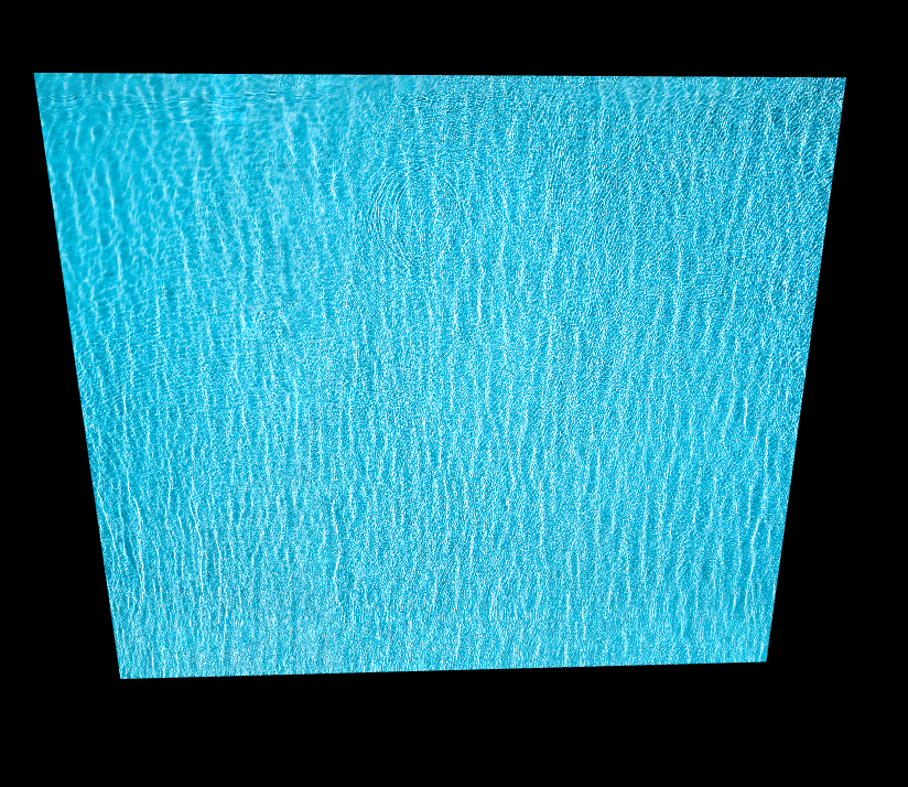
결국에는 너무 쉽게도 Mesh 의 Vertex 정보와, Normal 정보, 그리고 Vertex 들의 관계 (index) 정보들을 가지고 만들수 있다. 일단 Texture 를 준비해보자. 그리고 현재 Game Engine 에 올려보자. 아래의 Texture 는 물을 표현한 Texture 이다.
그리고 격자를 그리기위해서, 결국에는 Vertex 의 정보가 필요하다. 격자를 그리기위해나 Parameter 로서는 Width, Height, Stack, Slice 라고 보면 될것 같다.
Width & Height 는 격자의 총길이, 그리고 stack 몇개의 Box 를 위쪽으로 쌓을건지와, Slice 는 Width 에서 얼마나 자를건지를 표현한다.
코드는 따로 공유는 하지 않겠다, 하지만 격자는 아래와 같이 그려낼수 있다. 결국에는 평면이기 때문에 임의 Normal 값을 -z (모니터가 나를 바라보는 쪽) 으로 되어있고, 그리고 격자의 Vertex 의 정보는 Slice 와 Stack 으로 Point 를 Translation 해줬으며, 그리고 Index 들은 간단한 offset 으로 구현을 했었다.
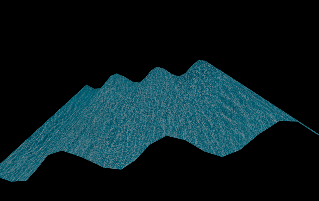
재밌으니까, 물결 Texture 니까, 물결을 나타내는 Texture 를 한번 구부려보자. z 축을 x 의 sin graph 로 그려내보자. 그리고 이거에대한 Normal 값도 따로 적용한다고 하면 두개의 Image 를 확인할수 있다. x 에 대한 변화량에 대한 z 값을 그려냈기때문에, 편미분을 통해서 결과값을 도출해낼수 있다.
이제껏 해본걸 종합해보자. Plane 도 만들어보았고, Box Mesh 도 만들어보았다. 근데 Cylinder 는? 사실 Cylinder 는 앞에 Grid 의 평면을 말아 놓은거라고 볼수 있다. 그렇다면, 어떻게 해야할까?가 고민일텐데, Texture 좌표 때문에 Vertex 를 + 1 을 해줘야한다. 그 이유는 Texture 좌표계 때문이다. (0~1) 로 반복되는거로 되어야하기때문에 그렇다.
그리고 앞서서 배웠듯이 Normal Vector 는 inverse transpose 값을 해줘야 Scale 값에 영향이 없는 결과를 가지고 올수 있다.
일단 이거는 살짝의 코드의 방향성을 생각을 해보면 좋을것 같다. 월드좌표계에서 Cylinder 를 만든다고 가정을 했을때, 화면 안으로 들어가는 좌표 z, Right Vector 는 X 축, Up Vector 는 Y 축이라고 생각을하고. 모델링을 만들때는 Y 축을 기준 회전 (즉 x-z 평면에서 만든다고 볼수있다.)
그렇다고 하면, 모든 Vertex 를 얼마나 회전을 하느냐에 따라서, 각도를 const float dTheta = -XM_2PI / float(sliceCount); 결국에는 얼마나 잘라내는지에 따른것에 따라서 더 부드러운 원동모형을 만들수 있을것 같다. 그리고 Y 축의 회전이다 보니, 모든 Vertex 를 Y 축을 통해서 Rotation 값을 누적해가면 된다.
그러면 위의 Radius 와 아래의 Radius 를 x-z 평면으로 시작점으로 해서 돌리면 된다. 결과는 아래와 같다. 원통을 그리려면 Vertex 의 정보를 SimpleMath 에 있는 CreateRotationY 로 충분히 해도 되지만, sin, cos 을 사용해서 원통을 만들어도 똑같은 결과를 나타낸다.
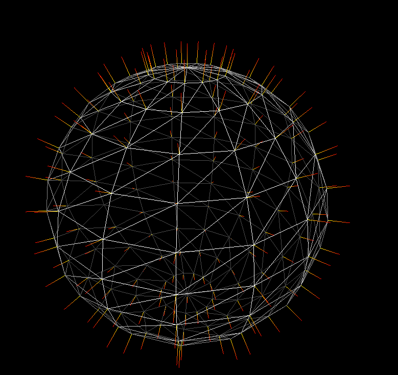
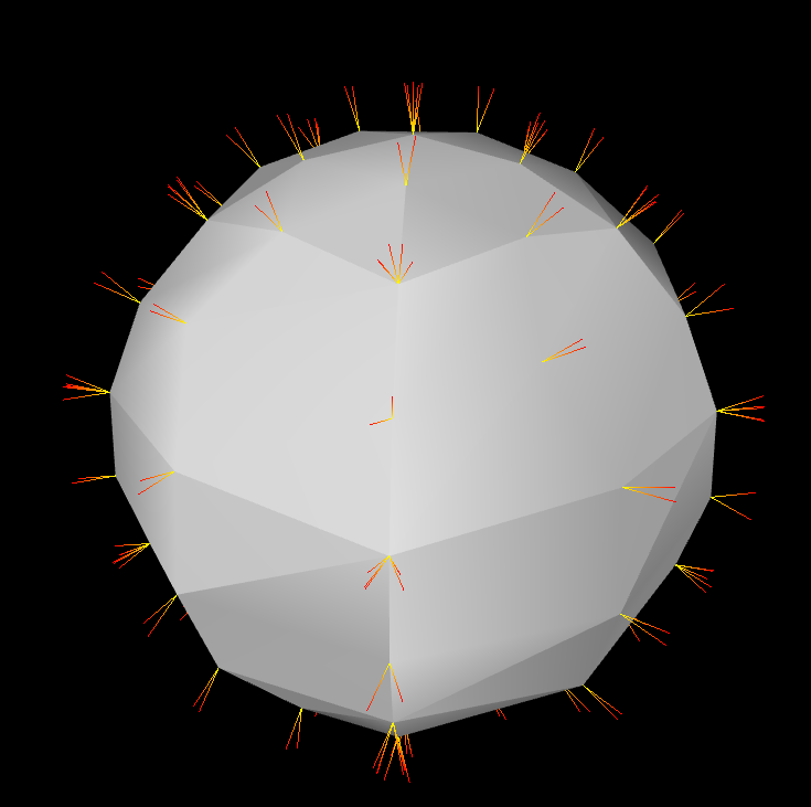
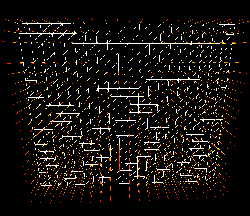
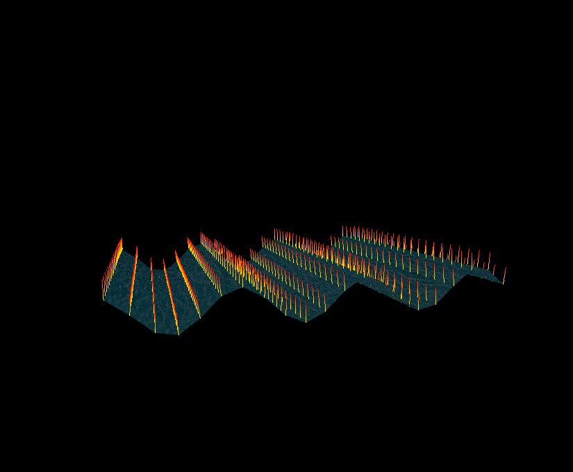
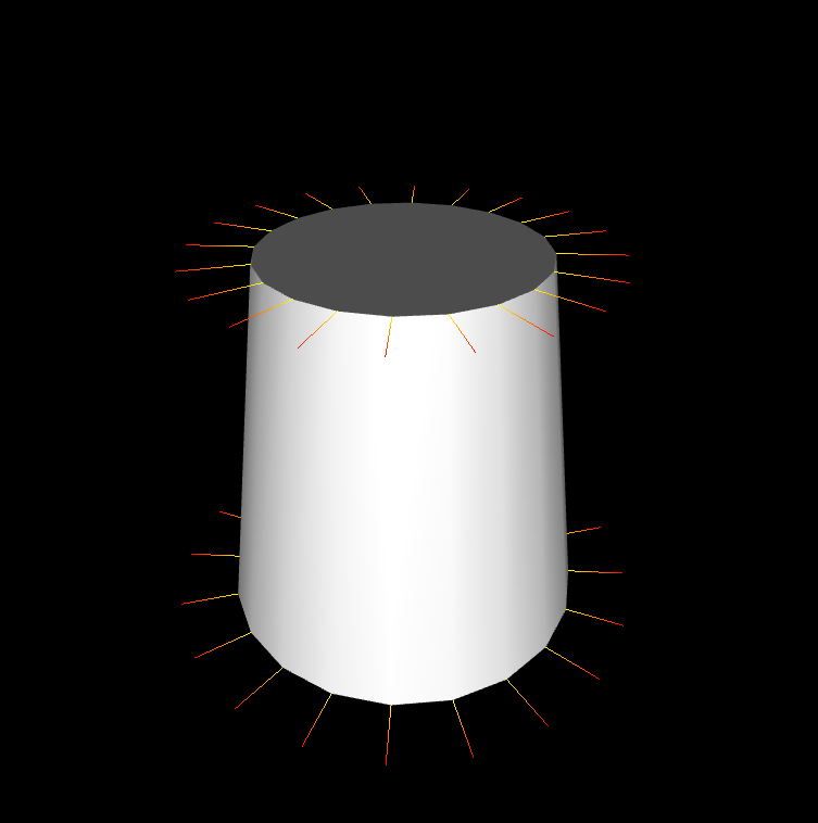
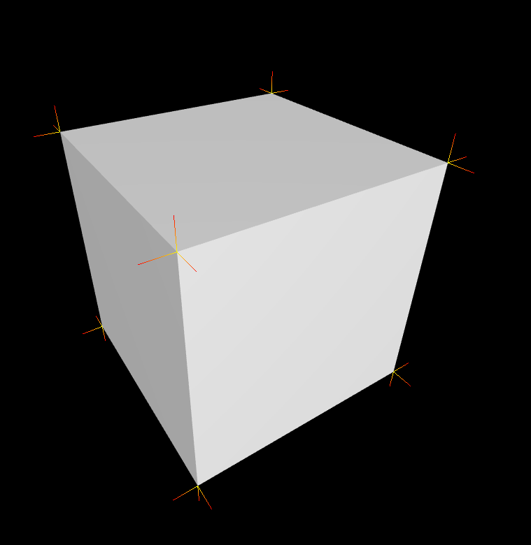
이전 Post 와 마찬가지로, 목적은 우리가 그려야할 Mesh 들의 Wireframe 도 봐야하지만, 각 면에 있는 Face Normal 값을 확인하는것도 Graphics Tool 로서는 중요하다. WireFrame 같은 경우는 DirectX 에서 는 RasterizerState 으로 해주었었다. 하지만 Normal 같은 경우 직접 그려야한다. 그래서 각 Vertex 별 Normal 값을 구하는게 중요하다. 물론 Unreal Engine 같은 경우 아래처럼 World Normal 을 볼수 있게끔 되어있다.
그렇다면 일단 만들어보자. 간단한 Box 의 Vertex 와 Normal 값들을 직접적으로 넣어주는 코드는 생략하겠다. 단 여기서 Point 는 HLSL 에서 어떻게 사용되는지를 알아보는게 더 중요하다.
일단 ConstantBuffer 에 들어가 있는걸로도 충분하니 아래의 코드를 일단 봐보자.
일단 Shader 코드를 살표 보자면, View 로 Transform 하기 이전에, Model 좌표계에서 의 Normal Vector 들을 World 좌표계로 구한다. 그런다음에, 시작점과 끝점을 확실히 하기위해서, texcoord 를 CPU 쪽에서 넘겨줄때 .x 값을 넘겨서 시작과 끝을 알려주는거를 넣어주면 될것 같다. 그리고 t 가 1 면 normal vector 의 원점 (노란색) 그리고 t 가 0 이면, normal vector 의 끝점인 (빨간색) 으로 표시할수 있게한다.
이제 CPU 쪽 작업을 해보자. CPU 에서 보내줄 정보는 GPU 에서의 보내줄 정보와 같다. CPU 쪽에서는 새로운 Normal 값들을 집어넣어야 하기에 정점 정보와 Normal 의 Indices 정보를 넣어서, Buffer 안에다가 채워넣어준다. 그리고 말했던 Normal 의 시작과 끝을 알리는 정보로서 texcoord 에 Attribute 로 집어 넣어준다. 마찬가지로 ConstantBuffer 도 Model, View, Projection 을 원하는 입맛에 맛게끔 집어넣어주면 될것 같다. 그리고 마지막으로 ConstantBuffer 를 Update 만해주면 내가 바라보는 시점에 따라서 Normal 도 같이 움직이는걸 확인할수 있다.
structMyVertexConstantBuffer{matrixmodel;matrixinvTranspose;matrixview;matrixprojection;}MyVertexConstantBufferm_MyVertexConstantData;ComPtr<ID3D11Buffer>m_vertexConstantBuffer;ComPtr<ID3D11Buffer>m_vertexBuffer;ComPtr<ID3D11Buffer>m_indexBuffer;ComPtr<ID3D11VertexShader>m_normalVertexShader;ComPtr<ID3D11PixelShader>m_normalPixelShader;UINTm_indexCount=0;//-----------------------------------------------------//// Init ()std::vector<Vertex>normalVertices;std::vector<uint16_t>normalIndices;for(size_ti=0;i<vertices.size();i++){autodata=verticies[i];data.texcoord.x=0.0f;normalVertices.push_back(data);data.texcoord.x=1.0f;normalVertices.push_back(data);normalIndices.push_back(uint16_t(2*i));normalIndices.push_back(uint16_t(2*i+1));}CreateVertexBuffer(normalVertices,m_vertexBuffer);m_indexCount=UINT(normalIndices.size());CreateIndexBuffer(normalIndicies,m_indexBuffer);CreateConstantBuffer(m_MyVertexConstantData,m_vertexConstantBuffer);// Then you need to Create Vetex / InputLayout & PixelShader to bind the resources.//-----------------------------------------------------//// Update ()// occluded the (M)odel(V)iew(P)rojection CalculationUpdateBuffer(m_MyVertexConstantData,m_vertexConstantBuffer);//-----------------------------------------------------//// Render()m_context->VSSetShader(m_normalVertexShader.Get(),0,0);ID3D11Buffer*pptr[1]={m_vertexConstantBuffer.Get()};m_context->VSSetConstantBuffers(0,1,pptr);m_context->PSSetShader(m_normalPixelShader.Get(),0,0);m_context->IASetVertexBuffers(0,1,>m_vertexBuffer.GetAddressOf(),&stride,&offset);m_context->IASetIndexBuffer(m_indexBuffer.Get(),DXGI_FORMAT_R16_UINT,0)m_context->IASetPrimitiveTopology(D3D11_PRIMITIVE_TOPOLOGY_LINELIST);m_context->DrawIndexed(m_indexCount,0,0);
결과는 아래와 같다.
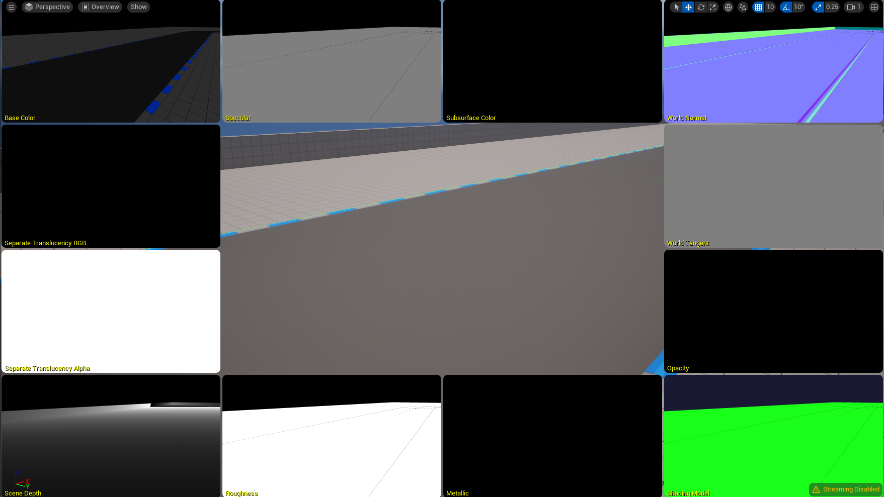
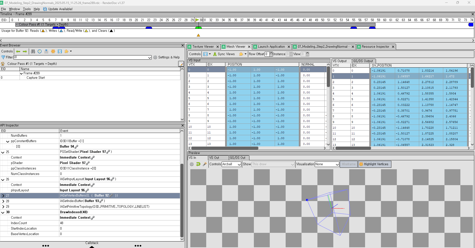
RenderDoc 으로도 돌려봐야하지 않겠냐? 싶어서, Vertex 의 Input 정보들을 확인할수 있다. 그리고 내가 어떠한 Parameter 로 넣어줬는지에 대한 State 들도 왼쪽에 명시 되어있다.
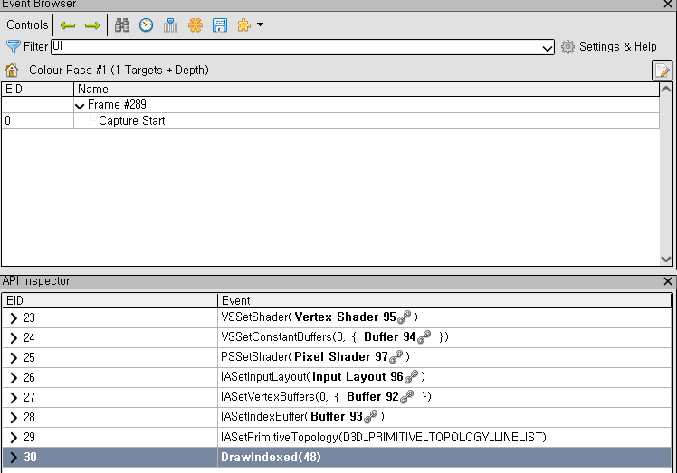
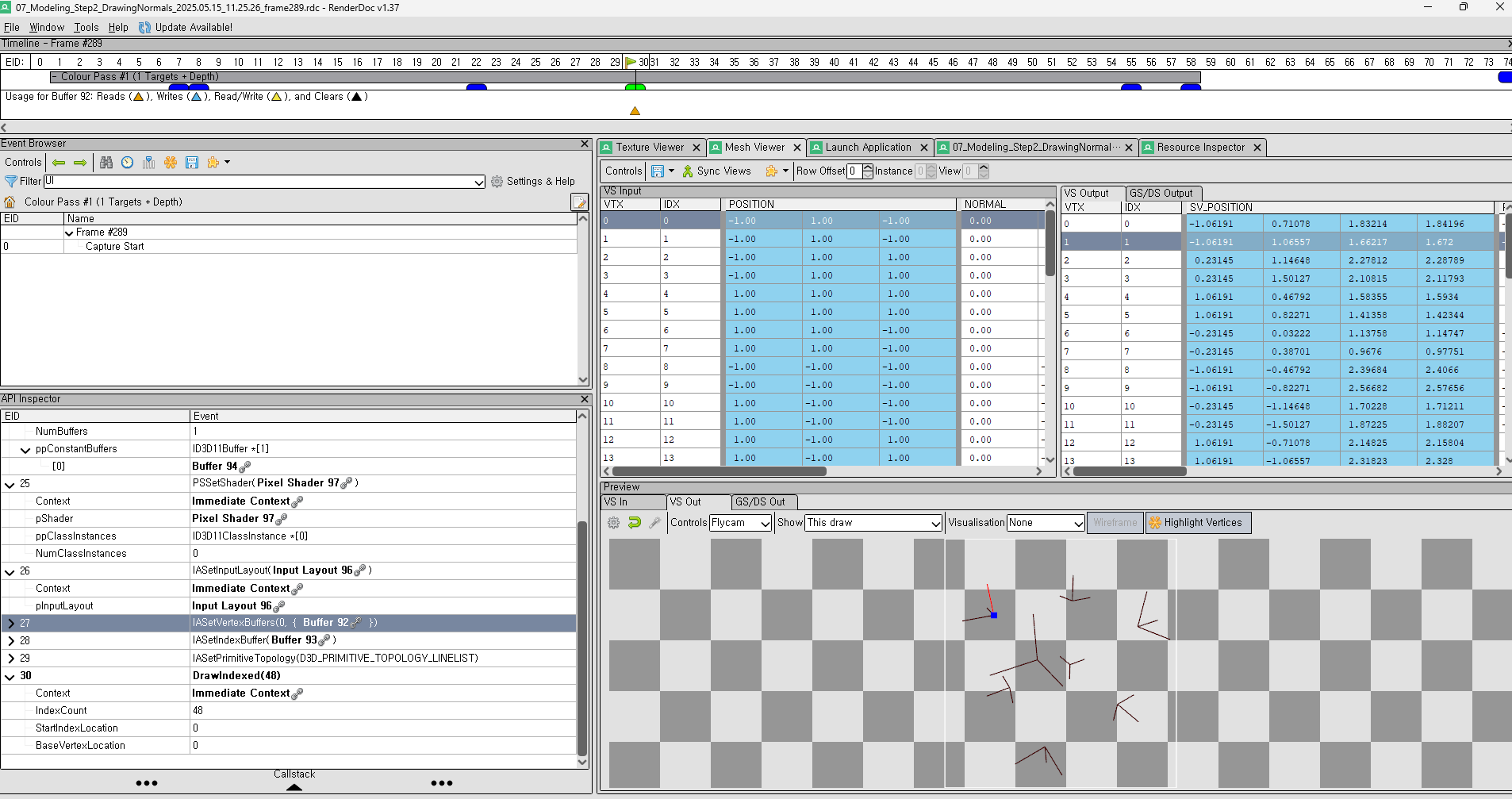
그리고 Vertex Shader 로 부터 Output 이 생성이 되면 아래와 같이 각 Vertex 과 면에 대해서 Normal 값이 나오는걸 확인할수 있다.
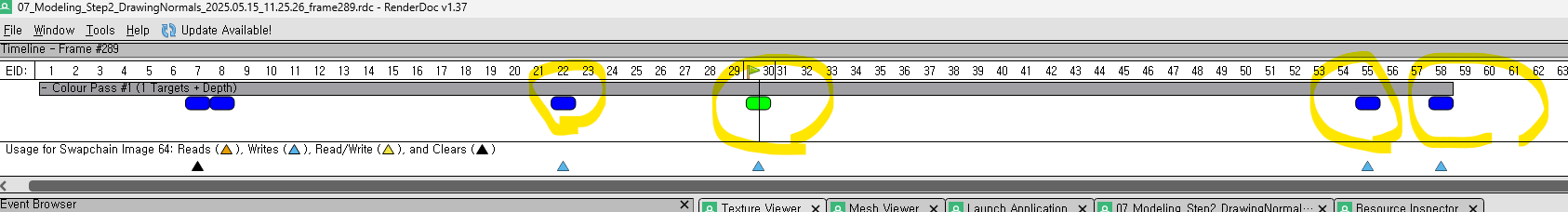
그리고 이건 DrawIndexed 의 호출을 동그라미 친것이다. ImGUI 도 쓰기때문에 저 뒤에 두번째는 ImGUI 가 현재 RenderTarget 에 DrawIndexed 를 해주고, 내가 Rendering 하고 싶은 결과는 노란색 두개 이다.
이렇게해서 RenderDoc 을 사용해서 검증을 하고 내가 Pipeline 에잘 넣었는지도 확인할수 있다.
결국에는 우리가 직접 Lighting 을 CPU 에서 계산하는게 아닌 GPU 에서 계산하도록 해야한다, 그럴려면 Shader Programming 으로 할수 있는 방법들을 찾아야한다.
일단 기본적인 어떤 Lighting 을 계산하기 위해서는 물체의 Normal 값이 필요하기 때문에, ModelViewProjection 이라는 Constant Buffer 에다가 InverseTransform 을 넣어줘야한다. 여기서 잠깐! 왜 Model 그대로 Normal 을 구하지 않는지를 물어볼수 있다. 그건 바로 Model 의 Scaling 이 변한다고 했을때, Normal 의 길이(크기)가 달라지기 때문에, Inverse Transpose Model Matrix 를 넣어줘야한다. 처음에는 위치값을 제거하고 (Translation), 그리고 .Invert().Transpose() 를 해주면, World Normal 값을 Shader 에서 구할수 있다.
자 일단 ConstantBuffer 를 Update 해주는 곳은 Render() 에서 매 Frame 별로 Update 를 해준다. 그러기때문에 아래의 방식처럼 CPU 에서 GPU 로 Data 넘길것들을 정의 해준다. 물론 이야기는 따로 하진 않겠지만, Model -> View -> Projection 으로 행렬을 곱하는데, 월드 좌표계에서의 Camera 의 위치를 구하기 위해서, m_pixelConstantBufferData.eyeWorld = Vector3::Transform(Vector3(0.0f), m_vertexConstantBufferData.view.Invert()); 이부분이 들어간거다.
structVertex{Vector3position;Vector3normal;Vector2texcoord;};structVertexConstantBuffer{Matrixmodel;MatrixinvTranspose;Matrixview;Matrixprojection;};// Render() -> Constant Buffer Updatem_vertexConstantBufferData.model=Matrix::CreateScale(m_modelScaling)*Matrix::CreateRotationX(m_modelRotation.x)*Matrix::CreateRotationY(m_modelRotation.y)*Matrix::CreateRotationZ(m_modelRotation.z)*Matrix::CreateTranslation(m_modelTranslation);m_vertexConstantBufferData.model=m_vertexConstantBufferData.model.Transpose();m_vertexConstantBufferData.invTranspose=m_vertexConstantBufferData.model.;m_vertexConstantBufferData.invTranspose.Translation(Vecctor3(0.0f));// get rid of translationm_vertexConstantBufferData.invTranspose=m_vertexConstantBufferData.invTranspose.Transpose().Invert()m_vertexConstantBufferData.view=Matrix::CreateRotationY(m_viewRot)*Matrix::CreateTranslation(0.0f,0.0f,2.0f);m_pixelConstantBufferData.eyeWorld=Vector3::Transform(Vector3(0.0f),m_vertexConstantBufferData.view.Invert());m_vertexConstantBufferData.view=m_vertexConstantBufferData.view.Transpose();
이렇게 필요한 Data 가 주어졌을떄, Lighting 기반 Bling Phong with Lambert equation 을 사용해서 Shader Programming 을 해야한다. 일단 CPU 쪽의 Data 를 정의 한다. 카메라의 위치와 어떤 Light 인지를 담는, Constant Buffer 를 사용하자. Lights 의 종류는 3 가지 (Directional Light, Point Light, Spotlight) 이렇게 나누어진다.
그리고 Render() 하는 부분에서, ConstantBuffer 값을 Update 를 한다. 빛의 종류에 따른 Update. Directional Light = 0, Point Light = 1, Spot Light = 2. 이렇게 되어있으며, 내가 필요한 Light 만 사용할수 있게끔 다른 Light 들을 꺼주는것이다. (.strength *= 0.0f)
가끔 우리는 어떤 Mesh를 사용하고 있는지, 그리고 그 Mesh가 얼마나 많은 삼각형으로 이루어져 있는지를 파악해야 할 필요가 있다.. 이는 성능 최적화나 실시간 렌더링 가능 여부를 평가할 때 중요하고 특히, 고해상도 Terrain이나 복잡한 조각상 같은 모델이 있는 경우 (물론 다른 stage 에서..), 런타임에서 모델을 사용할 수 있는지 판단하는 데 중요한 기준이 됩니다.
예를 들어, Unreal Engine의 Nanite System은 매우 많은 Vertex를 활용하여 고도로 디테일한 모델을 실시간으로 렌더링할 수 있다.. 이는 LOD(레벨 오브 디테일)를 효율적으로 관리하여 성능 저하 없이도 높은 품질의 그래픽을 제공할 수 있게 해줍니다. 그렇다면, 실제로 삼각형 개수를 확인하려면 어떻게 해야 할까요? 정답은 Rendering Pipeline의 상태를 확인하는 것입니다. 특히, Rasterizer 단계에서 어떻게 삼각형을 그릴 것인지 결정하는 RasterizerState를 통해 설정할 수 있다. 그리고 나중에 Rasterizer State 들을 만들어주면 된다.