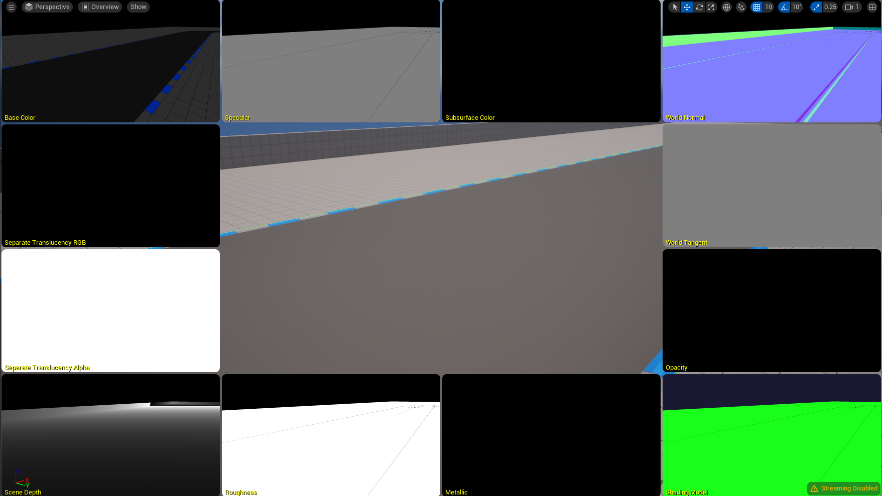
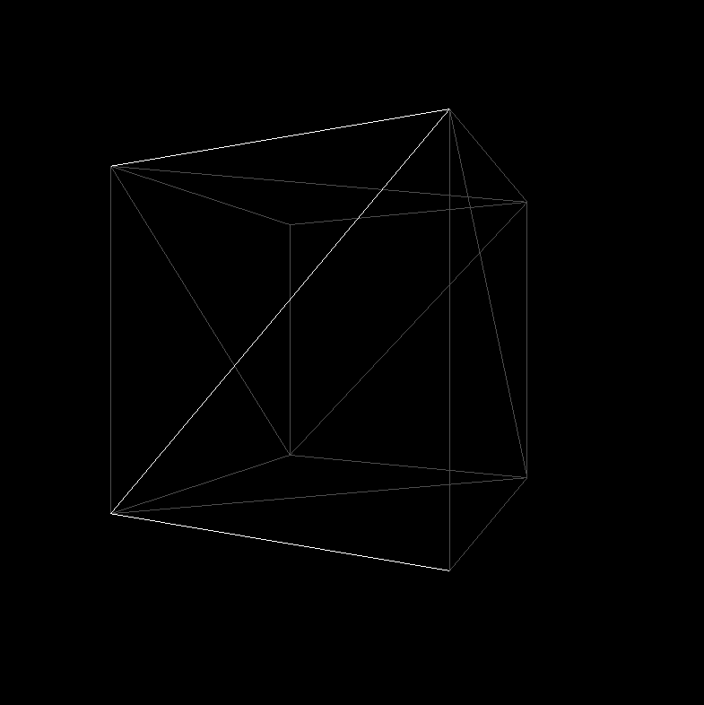
이전 Post 와 마찬가지로, 목적은 우리가 그려야할 Mesh 들의 Wireframe 도 봐야하지만, 각 면에 있는 Face Normal 값을 확인하는것도 Graphics Tool 로서는 중요하다. WireFrame 같은 경우는 DirectX 에서 는 RasterizerState 으로 해주었었다. 하지만 Normal 같은 경우 직접 그려야한다. 그래서 각 Vertex 별 Normal 값을 구하는게 중요하다. 물론 Unreal Engine 같은 경우 아래처럼 World Normal 을 볼수 있게끔 되어있다.

그렇다면 일단 만들어보자. 간단한 Box 의 Vertex 와 Normal 값들을 직접적으로 넣어주는 코드는 생략하겠다. 단 여기서 Point 는 HLSL 에서 어떻게 사용되는지를 알아보는게 더 중요하다.

일단 ConstantBuffer 에 들어가 있는걸로도 충분하니 아래의 코드를 일단 봐보자.

struct VertexShaderInput {
    float3 modelPos: POSITION;
    float3 normalModel: NORMAL;
    float2 texcoord : TEXCOORD0;
}

struct PixelShaderInput {
    float4 posProj : SV_POSITION;
    float3 posWorld: POSITION;
    float4 normalWorld : NORMAL;
    float2 texcoord : TEXCOORD;
    float3 color : COLOR;
}

cbuffer MyVertexConstantBuffer : register(b0)
{
    matrix model;
    matrix invTranspose;
    matrix view;
    matrix projection;
}

PixeShaderInput main(VertexShaderInput input) {
    PixelShaderInput output;
    float4 pos = float4(input.posModel, 1.0f);

    float4 normal = float4(input.normalModel, 0.0f);
    output.normalWorld = mul(normal, invTranspose).xyz;
    output.normalWorld = normalize(output.normalWorld);

    pos = mul(pos, model);

    float t = input.texcoord.x;

    pos.xyz += output.normalWorld * t * scale;

    output.posWorld = pos.xyz;

    pos = mul(pos, view);
    pos = mul(pos, projection);

    output.posProj = pos;
    output.texcoord = input.texcoord;

    output.color = float3(1.0, 1.0, 0.0) * (1.0 - t) + float3(1.0, 0.0, 0.0) * t;

    return output;
}

float4 main(PixelShaderInput input) : SV_TARGET
{
    return float4(input.color, 1.0f);
}

일단 Shader 코드를 살표 보자면, View 로 Transform 하기 이전에, Model 좌표계에서 의 Normal Vector 들을 World 좌표계로 구한다. 그런다음에, 시작점과 끝점을 확실히 하기위해서, texcoord 를 CPU 쪽에서 넘겨줄때 .x 값을 넘겨서 시작과 끝을 알려주는거를 넣어주면 될것 같다. 그리고 t 가 1 면 normal vector 의 원점 (노란색) 그리고 t 가 0 이면, normal vector 의 끝점인 (빨간색) 으로 표시할수 있게한다.

이제 CPU 쪽 작업을 해보자. CPU 에서 보내줄 정보는 GPU 에서의 보내줄 정보와 같다. CPU 쪽에서는 새로운 Normal 값들을 집어넣어야 하기에 정점 정보와 Normal 의 Indices 정보를 넣어서, Buffer 안에다가 채워넣어준다. 그리고 말했던 Normal 의 시작과 끝을 알리는 정보로서 texcoord 에 Attribute 로 집어 넣어준다. 마찬가지로 ConstantBuffer 도 Model, View, Projection 을 원하는 입맛에 맛게끔 집어넣어주면 될것 같다. 그리고 마지막으로 ConstantBuffer 를 Update 만해주면 내가 바라보는 시점에 따라서 Normal 도 같이 움직이는걸 확인할수 있다.

struct MyVertexConstantBuffer
{
    matrix model;
    matrix invTranspose;
    matrix view;
    matrix projection;
}

MyVertexConstantBuffer m_MyVertexConstantData;
ComPtr<ID3D11Buffer> m_vertexConstantBuffer;
ComPtr<ID3D11Buffer> m_vertexBuffer;
ComPtr<ID3D11Buffer> m_indexBuffer;
ComPtr<ID3D11VertexShader> m_normalVertexShader;
ComPtr<ID3D11PixelShader> m_normalPixelShader;
UINT m_indexCount = 0;

//-----------------------------------------------------//
// Init ()
std::vector<Vertex> normalVertices;
std::vector<uint16_t> normalIndices;
for (size_t i = 0; i < vertices.size(); i++){
    auto data = verticies[i];
    data.texcoord.x = 0.0f;
    normalVertices.push_back(data);
    data.texcoord.x = 1.0f;
    normalVertices.push_back(data);

    normalIndices.push_back(uint16_t(2*i));
    normalIndices.push_back(uint16_t(2*i + 1));
}

CreateVertexBuffer(normalVertices, m_vertexBuffer);
m_indexCount = UINT(normalIndices.size());
CreateIndexBuffer(normalIndicies, m_indexBuffer);
CreateConstantBuffer(m_MyVertexConstantData, m_vertexConstantBuffer);

// Then you need to Create Vetex / InputLayout & PixelShader to bind the resources.

//-----------------------------------------------------//
// Update ()
// occluded the (M)odel(V)iew(P)rojection Calculation
UpdateBuffer(m_MyVertexConstantData, m_vertexConstantBuffer);

//-----------------------------------------------------//
// Render()
m_context->VSSetShader(m_normalVertexShader.Get(), 0, 0);
ID3D11Buffer *pptr[1] = {m_vertexConstantBuffer.Get()};

m_context->VSSetConstantBuffers(0, 1, pptr);
m_context->PSSetShader(m_normalPixelShader.Get(), 0, 0);
m_context->IASetVertexBuffers(
    0, 1, >m_vertexBuffer.GetAddressOf(), &stride,
    &offset);
m_context->IASetIndexBuffer(m_indexBuffer.Get(),
                            DXGI_FORMAT_R16_UINT, 0)
m_context->IASetPrimitiveTopology(D3D11_PRIMITIVE_TOPOLOGY_LINELIST);
m_context->DrawIndexed(m_indexCount, 0, 0);

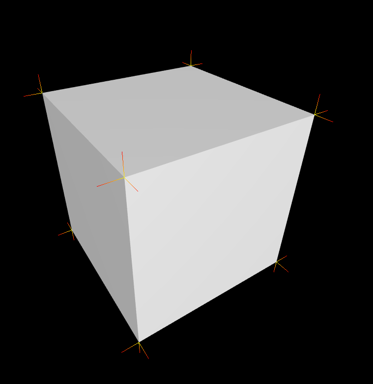
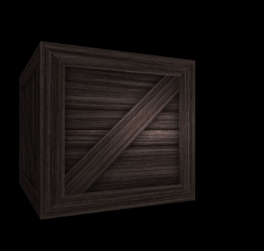
결과는 아래와 같다.

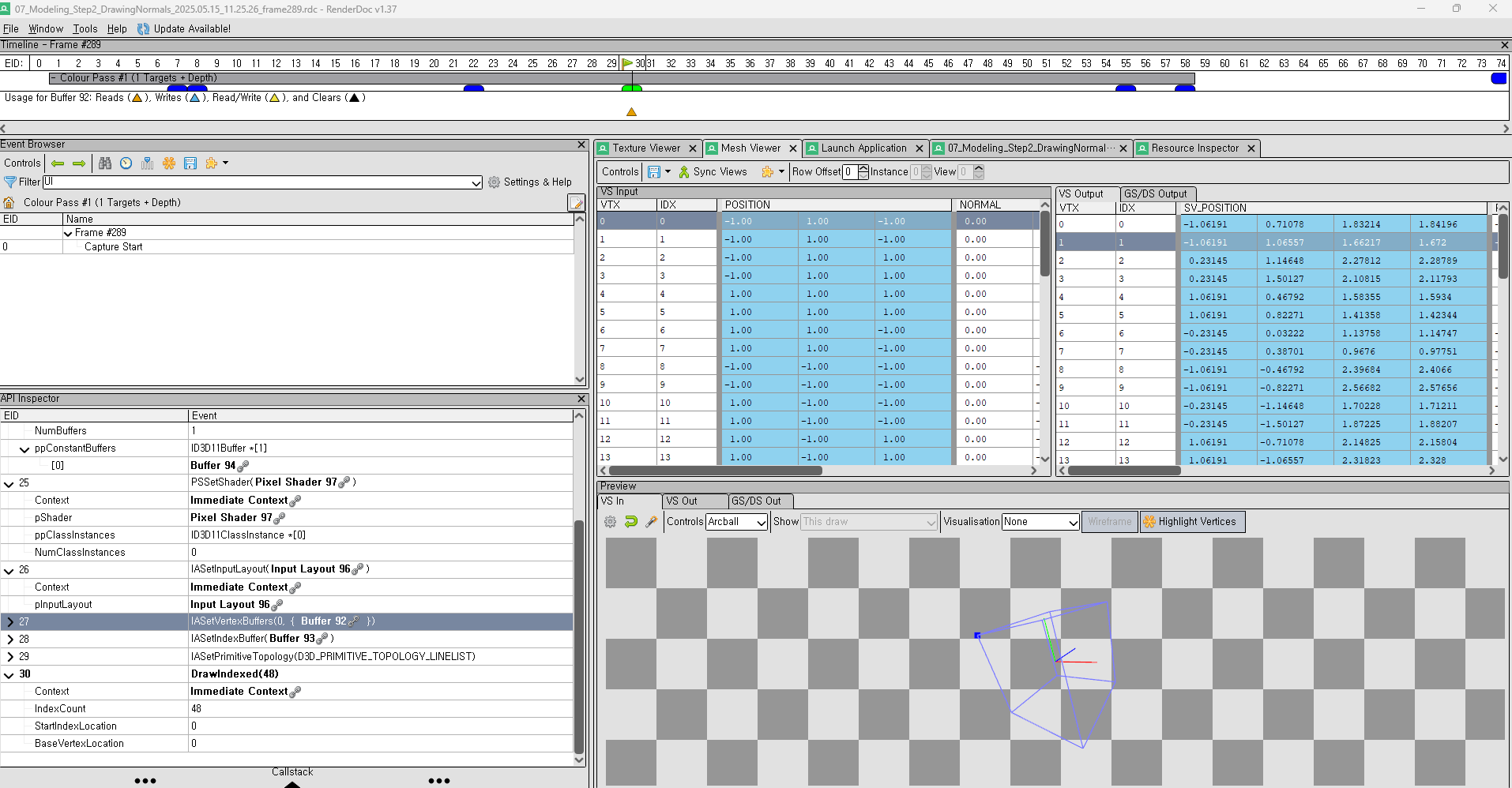
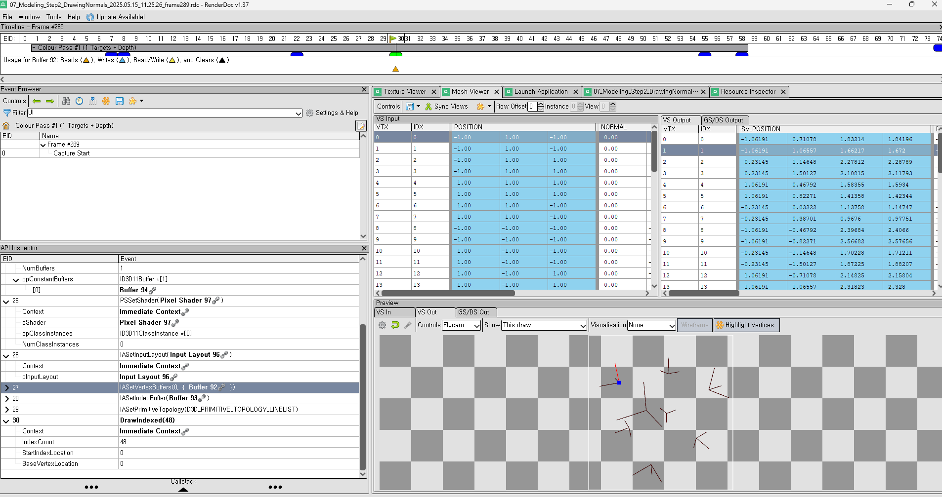
RenderDoc 으로도 돌려봐야하지 않겠냐? 싶어서, Vertex 의 Input 정보들을 확인할수 있다. 그리고 내가 어떠한 Parameter 로 넣어줬는지에 대한 State 들도 왼쪽에 명시 되어있다.

그리고 Vertex Shader 로 부터 Output 이 생성이 되면 아래와 같이 각 Vertex 과 면에 대해서 Normal 값이 나오는걸 확인할수 있다.

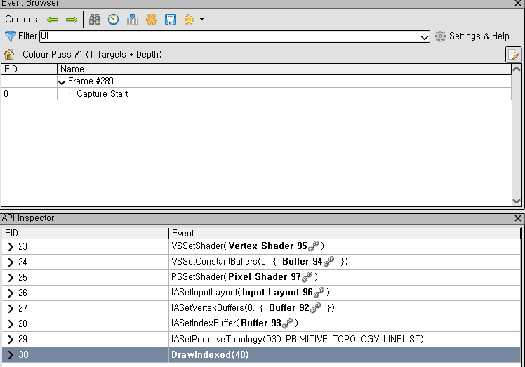
그리고 이건 DrawIndexed 의 호출을 동그라미 친것이다. ImGUI 도 쓰기때문에 저 뒤에 두번째는 ImGUI 가 현재 RenderTarget 에 DrawIndexed 를 해주고, 내가 Rendering 하고 싶은 결과는 노란색 두개 이다.

이렇게해서 RenderDoc 을 사용해서 검증을 하고 내가 Pipeline 에잘 넣었는지도 확인할수 있다.

결국에는 우리가 직접 Lighting 을 CPU 에서 계산하는게 아닌 GPU 에서 계산하도록 해야한다, 그럴려면 Shader Programming 으로 할수 있는 방법들을 찾아야한다.

일단 기본적인 어떤 Lighting 을 계산하기 위해서는 물체의 Normal 값이 필요하기 때문에, ModelViewProjection 이라는 Constant Buffer 에다가 InverseTransform 을 넣어줘야한다. 여기서 잠깐! 왜 Model 그대로 Normal 을 구하지 않는지를 물어볼수 있다. 그건 바로 Model 의 Scaling 이 변한다고 했을때, Normal 의 길이(크기)가 달라지기 때문에, Inverse Transpose Model Matrix 를 넣어줘야한다. 처음에는 위치값을 제거하고 (Translation), 그리고 .Invert().Transpose() 를 해주면, World Normal 값을 Shader 에서 구할수 있다.

자 일단 ConstantBuffer 를 Update 해주는 곳은 Render() 에서 매 Frame 별로 Update 를 해준다. 그러기때문에 아래의 방식처럼 CPU 에서 GPU 로 Data 넘길것들을 정의 해준다. 물론 이야기는 따로 하진 않겠지만, Model -> View -> Projection 으로 행렬을 곱하는데, 월드 좌표계에서의 Camera 의 위치를 구하기 위해서, m_pixelConstantBufferData.eyeWorld = Vector3::Transform(Vector3(0.0f), m_vertexConstantBufferData.view.Invert()); 이부분이 들어간거다.

struct Vertex {
    Vector3 position;
    Vector3 normal;
    Vector2 texcoord;
};

struct VertexConstantBuffer {
    Matrix model;
    Matrix invTranspose;
    Matrix view;
    Matrix projection;
};

// Render() -> Constant Buffer Update
m_vertexConstantBufferData.model =
    Matrix::CreateScale(m_modelScaling) *
    Matrix::CreateRotationX(m_modelRotation.x) *
    Matrix::CreateRotationY(m_modelRotation.y) *
    Matrix::CreateRotationZ(m_modelRotation.z) *
    Matrix::CreateTranslation(m_modelTranslation);

m_vertexConstantBufferData.model =
        m_vertexConstantBufferData.model.Transpose();

m_vertexConstantBufferData.invTranspose = m_vertexConstantBufferData.model.;
m_vertexConstantBufferData.invTranspose.Translation(Vecctor3(0.0f)); // get rid of translation
m_vertexConstantBufferData.invTranspose = m_vertexConstantBufferData.invTranspose.Transpose().Invert()

m_vertexConstantBufferData.view = Matrix::CreateRotationY(m_viewRot) * Matrix::CreateTranslation(0.0f, 0.0f, 2.0f);

m_pixelConstantBufferData.eyeWorld = Vector3::Transform(
    Vector3(0.0f), m_vertexConstantBufferData.view.Invert());
m_vertexConstantBufferData.view =
    m_vertexConstantBufferData.view.Transpose();

이렇게 필요한 Data 가 주어졌을떄, Lighting 기반 Bling Phong with Lambert equation 을 사용해서 Shader Programming 을 해야한다. 일단 CPU 쪽의 Data 를 정의 한다. 카메라의 위치와 어떤 Light 인지를 담는, Constant Buffer 를 사용하자. Lights 의 종류는 3 가지 (Directional Light, Point Light, Spotlight) 이렇게 나누어진다.

#define MAX_LIGHTS 3
struct PixelConstantBuffer {
    Vector3 eyeWorld; 
    bool dummmy;
    Material material;
    Light lights[MAX_LIGHTS];
}

struct Light {
    Vector3 strength = Vector3(1.0f);             
    float fallOffStart = 0.0f;                     
    Vector3 direction = Vector3(0.0f, 0.0f, 1.0f); 
    float fallOffEnd = 10.0f;                    
    Vector3 position = Vector3(0.0f, 0.0f, -2.0f); 
    float spotPower = 1.0f;                        
};

struct Material {
    Vector3 ambient = Vector3(0.1f);  
    float shininess = 1.0f;           
    Vector3 diffuse = Vector3(0.5f);  
    float dummy1;                     
    Vector3 specular = Vector3(0.5f); 
    float dummy2;                     
};

class Renderer()
public:
    ComPtr<ID3D11Buffer> m_pixelShaderConstantBuffer;
    ComPtr<ID3D11Texture2D> m_texture;
    ComPtr<ID3D11ShaderResourceView> m_textureResourceView;
    PixelConstantBuffer m_pixelConstantBufferData;
    float m_materialDiffuse = 1.0f;
    float m_materialSpecular = 1.0f;

그리고 Render() 하는 부분에서, ConstantBuffer 값을 Update 를 한다. 빛의 종류에 따른 Update. Directional Light = 0, Point Light = 1, Spot Light = 2. 이렇게 되어있으며, 내가 필요한 Light 만 사용할수 있게끔 다른 Light 들을 꺼주는것이다. (.strength *= 0.0f)

m_pixelConstantBufferData.material.diffuse = Vector3(m_materialDiffuse);
m_pixelConstantBufferData.material.specular = Vector3(m_materialSpecular);
for (int i = 0; i < MAX_LIGHTS; i++) {
    if (i != m_lightType) {
        m_pixelConstantBufferData.lights[i].strength *= 0.0f;
    } else {
        m_pixelConstantBufferData.lights[i] = m_lightFromGUI;
    }
}

CPU 쪽에서 Data 를 만들었다면 이제 GPU 에다가도 똑같이 Resource Binding 을위해서 정의를 한다.

// Common.hlsli
#define MAX_LIGHTS 3 
#define NUM_DIR_LIGHTS 1
#define NUM_POINT_LIGHTS 1
#define NUM_SPOT_LIGHTS 1

struct Material
{
    float3 ambient;
    float shininess;
    float3 diffuse;
    float dummy1; 
    float3 specular;
    float dummy2;
};

struct Light
{
    float3 strength;
    float fallOffStart;
    float3 direction;
    float fallOffEnd;
    float3 position;
    float spotPower;
};

float CalcAttenuation(float d, float falloffStart, float falloffEnd)
{
    // Linear falloff
    return saturate((falloffEnd - d) / (falloffEnd - falloffStart));
}

float3 BlinnPhong(float3 lightStrength, float3 lightVec, float3 normal,
                   float3 toEye, Material mat)
{
    float3 halfway = normalize(toEye + lightVec);
    float hdotn = dot(halfway, normal);
    float3 specular = mat.specular * pow(max(hdotn, 0.0f), mat.shininess);
    return mat.ambient + (mat.diffuse + specular) * lightStrength;
}

float3 ComputePointLight(Light L, Material mat, float3 pos, float3 normal, float3 toEye) {
    float3 lightVec = L.position - pos;
    float d = length(lightVec);

    if (d > L.fallOffEnd) {
        return float3(0.0, 0.0, 0.0);
    } else {
        lightVec /= d;
        float ndotl = max(dot(ligthVec, normal), 0.0f); // Light STrength related
        float3 lightStrength = L.strength * ndotl;
        float attenutationFactor = CalcAttenuation(d, L.fallOffStart, L.fallOffEnd);
        lightStrength *= attenutationFactor;
        return BlingPhong(lightStrength, lightVec, normal, toEye, mat);
    }
}

위를 코드를 사용해서, 각각의 Directional Light / Point Light / Spot Light 를 구현할수 있을것이다. 추가적으로 Spot Light 같은경우에는, Pow 를 사용해서, Alpha 값을 제곱을 해주는 작업도 필요하다.

Resource

• ScratchPixel

가끔 우리는 어떤 Mesh를 사용하고 있는지, 그리고 그 Mesh가 얼마나 많은 삼각형으로 이루어져 있는지를 파악해야 할 필요가 있다.. 이는 성능 최적화나 실시간 렌더링 가능 여부를 평가할 때 중요하고 특히, 고해상도 Terrain이나 복잡한 조각상 같은 모델이 있는 경우 (물론 다른 stage 에서..), 런타임에서 모델을 사용할 수 있는지 판단하는 데 중요한 기준이 됩니다.

예를 들어, Unreal Engine의 Nanite System은 매우 많은 Vertex를 활용하여 고도로 디테일한 모델을 실시간으로 렌더링할 수 있다.. 이는 LOD(레벨 오브 디테일)를 효율적으로 관리하여 성능 저하 없이도 높은 품질의 그래픽을 제공할 수 있게 해줍니다. 그렇다면, 실제로 삼각형 개수를 확인하려면 어떻게 해야 할까요? 정답은 Rendering Pipeline의 상태를 확인하는 것입니다. 특히, Rasterizer 단계에서 어떻게 삼각형을 그릴 것인지 결정하는 RasterizerState를 통해 설정할 수 있다. 그리고 나중에 Rasterizer State 들을 만들어주면 된다.

// Render 
ComPtr<ID3D11RasterizerState> _rasterizerState;
m_context->RSSetStet(_rasterizerState);

// INIT()
D3D11_RASTERIZER_DESC rastDesc;
ZeroMemory(&rastDesc, sizeof(D3D11_RASTERIZER_DESC)); 
m_OnWireFrame ? rastDesc.FillMode = D3D11_FILL_MODE::D3D11_FILL_WIREFRAME : rastDesc.FillMode = D3D11_FILL_MODE::D3D11_FILL_SOLID;
rastDesc.CullMode = D3D11_CULL_MODE::D3D11_CULL_NONE;
rastDesc.FrontCounterClockwise = false;
rastDesc.DepthClipEnable = true; 
m_device->CreateRasterizerState(&rastDesc,
                                 m_solidRasterizerSate.GetAddressOf());
 
m_device->CreateRasterizerState(&rastDesc,
                                 m_wireRasterizerSate.GetAddressOf());

물론 더나아가서 고품질의 그림을 그릴수도 있지만, 일단 WireFrame 을 그리는거까지 해보는것이 중요한것 같다. 결과는 아래와 같다.

내가 Build System 을 고려하다가 정리를 해본다.

지원 플랫폼 및 유연성

• Premake: 주로 Visual Studio, Xcode, GNU Make를 타겟으로 사용하며, 게임 엔진이나 그래픽 라이브러리 개발에 많이 사용됩니다.
• CMake: 거의 모든 플랫폼과 빌드 시스템을 지원합니다. 특히 Ninja와 함께 사용할 때 빌드 속도가 매우 빠릅니다.

  생태계와 커뮤니티 지원

• Premake: 게임 엔진 및 일부 그래픽 라이브러리에서 주로 사용됩니다. 대표적으로 LunaEngine이나 Unreal Engine에서 사용합니다.
• CMake: 오픈소스 프로젝트에서 표준으로 사용됩니다. 예를 들어 LLVM, Qt, OpenCV 등이 CMake를 사용

I’m currently working on my own game engine, called Luna Game Engine. Sometimes, the workload can feel overwhelming, especially when balancing personal projects and portfolio building. I find that taking a break and reflecting helps me maintain focus and productivity.

While working on Luna, I often draw inspiration from existing game engines like Unreal Engine, Unity, and FrostBite. Each of these engines has a distinct philosophy and approach to game development. For example, Unity is particularly focused on multi-platform support, which makes it versatile for mobile, console, and desktop applications. There’s a great video on YouTube that outlines Unity’s roadmap and how they plan to evolve the engine.

One remarkable feature of Unreal Engine is its support for large-scale triangle meshes through Nanite. However, I am a bit concerned about the runtime performance when loading these heavy meshes. While the visuals are undeniably impressive, maintaining performance is always a critical consideration.

Unity’s collaboration with Zyva is also noteworthy, especially when it comes to realistic facial animations. The demo shows incredibly vivid muscle movements that mimic human expressions. This kind of technology could significantly impact the VR industry and even healthcare applications.

Personally, I have a soft spot for FrostBite, as I have enjoyed the Battlefield series for years. I also find it fascinating how the engine has evolved, especially for FIFA. In older versions, scoring from long-distance shots was quite easy, but recent iterations have introduced more nuanced physics and player attributes, making gameplay more realistic. Small details, like players sweating, might seem minor, but they reflect just how far game engines have come in terms of visual fidelity and realism.

As I continue developing Luna Game Engine, I aim to incorporate some of the strengths I admire in these established engines while maintaining my own vision. Taking time to study how industry leaders approach engine design helps me make more informed decisions about Luna’s features and structure.

The Vulkan is the graphical API made by Khronos providing the better abstraction on newer graphic cards. This API outperform? the Direct3D and OpenGL by explaining what it perform. The idea of the Vulkan is similar to the Direct3D12 and Metal, but Vulkan is cross-platform, and it can be used and developed in Linux or Window Environment.

However, the drawback of this could be is there will be many detailed procedure while using the Vulkan API, such as creating the buffer frame, managing the memory for buffer and texture image objects. That means we would have to set up properly on application. I realized that the Vulkan is not for everyone, it is only for people who’s passionate on Computer Graphics Area. The current trends for computer graphics in Game Dev, they are switching the DirectX or OpenGL to Vulkan : Lists of Game made by Vulkan. One of the easier approach could be is to learn and play the computer graphics inside of Unreal Engine and Unity.

By designing from scratch for the latest graphics architecture, Vulkan can benefit from improved performance by eliminating bottlenecks with multi-threading support from CPUs and providing programmers with more control for GPUs. Reducing driver overhead by allowing programmers to clearly specify intentions using more detailed APIs, and allow multiple threads to create and submit commands in parallel and Reducing shader compilation inconsistencies by switching to a standardized byte code format with a single compiler. Finally, it integrates graphics and computing into a single API to recognize the general-purpose processing capabilities of the latest graphics cards.

There are three preconditions to follow

• Vulkan (NVIDA, AMD, Intel) compatible graphic cards and drivers
• Expereince in C++ ( RAII, initializer_list, Modern C++11)
• Compiler above C++17 (Visual Studio 2017, GCC 7+, Clang 5+)
• 3D computer Graphics Experience

How to install Vulkan on Visual Studio Code

Have to figure this out later on.

• How to build c++ code in visual studio code
• How to set the environment in visual studio code

Vulkan Componenet

Resources:

• Vulkan Tutorial
• Vulkan Tutorial Youtube-1
• Vulkan Tutorial Youtube-2
• Vulkan Tutorial Youtube-3
• Vulkan Introduction

This is just a graphics resource to learn DirectX

• DirectX Tutorial.com
• Braynzar Soft
• Rastertek.com
• ChillTomatoNoodle Youtube
• Cherno
• Learning Vulkan Github Repo
• MoltenVK Github Repo
• ImGUI - DirectX12
• ImGUI - Vulkan
• Mega3D

Limitation on Vision Transformer (ViT)

While Vision Transformers (ViT) have shown strong performance in image classification. There are several limitations that arise when applying them to more and various computer vision tasks.

1. Fixed Patch Size & Lack of Local Content

ViT splits the image into fixed-size patches (e.g., 16x16), regardless of the underlying content

As a results:

• The model may attent to meaningless or background regions (e.g white pixels) with no semantic values
• If important visual elements are split across patch boundaries, local similarity between pixels is lost

Maybe the example I can think of is, a small object like a bird might get split between patches, causing the network to miss its continuity entirely.

2. Poor Handling of Scale Variations

ViT lacks mechanisms to handle scale variablity in visual tokens. In real-world images:

• A bird could occupy 200x200 or just 20x20, but both should still be recognized as “a bird”
• Without scale-awareness, the model struggles to generalize across different object sizes.

3. Quadratic Complexity

ViT’s self-attention has quadratic complexity with respect to the number of patches (i.e., ( O(n^2) )).

This becomes computationally expensive for high-resolution images commonly found in practice (e.g., 1920×1080).

4. Limited to Classification Tasks

ViT was initially designed for image classification, but many vision applications require more:

• Object Detection: Unlike language tokens, visual elements vary widely in size and spatial distribution.
• Semantic Segmentation: Image resolution is much higher than text sequences, requiring dense predictions across pixels.

Solution & Architecture: Hierarchical Structure & Shifted Window Attention

• A pyramid-like hierarchical structure, inspired by CNNs and U-Net
• Shifted window-based local self-attention, which allows the model to:
  • Capture local context efficiently
  • Reduce computation to linear complexity with respect to image size
  • Scale well to high-resolution and dense prediction tasks

These architectural choices allow Transformers to be applied beyond classification—including detection and segmentation

A General Transformer Backbone for Vision

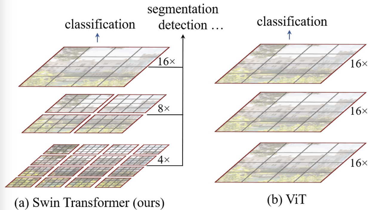
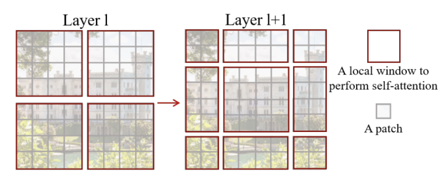
The diagram above illustrates the general structure of a Transformer-based vision backbone. The Swin Transformer begins by splitting the input image into small non-overlapping patches (gray outlines) and gradually builds up hierarchical representations by merging neighboring patches at deeper layers—similar to CNNs.

Local Self-Attention with Shifted Windows

To reduce computational complexity, Swin Transformer performs self-attention within non-overlapping windows (red outlines) rather than across the entire image.

• These windows are fixed in size (e.g., 4×4 patches).
• Attention is calculated only within each window, not globally.
• As a result, computational complexity becomes linear with respect to image size, instead of quadratic.

This window-based local attention allows the model to efficiently process images of various sizes, since the number of windows scales with the image size.

Example: Window and Patch Hierarchy

• Suppose the input image is divided into 16×16 windows, each window containing 4×4 patches.
• Within each 4×4 window:
  • Self-attention is computed locally, without looking outside the window.
• In deeper layers:
  • Neighboring patches are merged (e.g., combining 2×2 patches).
  • This reduces the total number of patches by a factor of 4, while increasing the spatial resolution of each patch (i.e., width × 2 and height × 2).

This hierarchical merging process enables the model to learn increasingly abstract and global features, while maintaining efficiency and scalability.

Multi-head Self-Attention in Swin Transformer

In Swin Transformer, attention is applied locally within windows. However, instead of applying the same partitioning across all layers, it introduces a clever mechanism:
Shifted Windows, which allows the model to connect neighboring windows and capture richer context. Each patch in a window shares the same key set, which not only simplifies computation but also improves memory access efficiency—crucial for hardware acceleration as explain furthermore.

Notably, all windows in Swin are non-overlapping.

W-MSA (Window-based Multi-head Self-Attention)

In Layer 1 of the Swin Transformer block (left side of the original figure above), the image is divided into non-overlapping windows. Self-attention is applied within each window only, making it a local attention mechanism. This is referred to as W-MSA.

SW-MSA (Shifted Window-based Multi-head Self-Attention)

In Layer 2 (right side of the original figure), the windows are shifted relative to the previous layer. This allows self-attention to be computed across window boundaries, connecting adjacent regions. While traditional sliding windows can also cover neighboring areas, shifted windows maintain efficiency while introducing inter-window connections, enabling the model to capture global interactions gradually.

Traditional Multi-head Self-Attention (MSA) computes attention globally across all tokens in an image. While this enables long-range dependencies, it comes with a significant computational cost.

Before, the complexity of global self-attenion is:

MSA: Ω(MSA) = 4 * h * w * C^2 + 2 * (h * w)^2 * C

Where:

• h, w = height and width of the feature map
• C = number of channels

But there is a problem with this, if the input resolution increases, the quadratic term grows dramatically - making it inefficient for high-resolution images.

To address this, Window-based Multi-head Self-Attention (W-MSA) restricts attention to local windows of size M × M. Its complexity is:

W-MSA: Ω(W-MSA) = 4 * h * w * C^2 + 2 * M^2 * h * w * C

Here, M is a fixed window size (e.g., 7), making this approach linear in terms of image size. This dramatically reduces computational cost while retaining performance in local contexts.

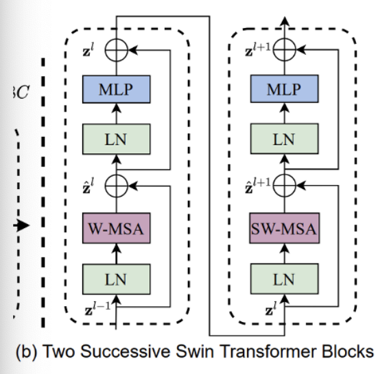
Also, the each swin transformer block consists of:

• A W-MSA or SW-MSA module
• A two-layer MLP with GELU activation
• Layer Normalization before each sub-layer
• A residual connection (skip connection) applied after each block

Model Architecture

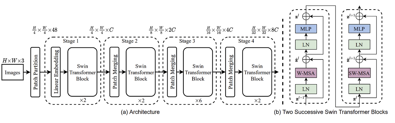
The figure above illustrates the overall architecture of the Swin Transformer. Here’s how the input image is processed step-by-step:

1. Patch Partitioning
   The input image is first split into non-overlapping patches of size 4×4, resulting in patch tokens of shape 4×4×3. Each patch is then flattened and passed through a Linear Projection to form an embedding vector.

2. Linear Embedding
   These patch vectors are embedded into a fixed-dimensional space using a learnable linear layer. This prepares them for the Transformer blocks that follow.

3. Transformer Blocks (Stage 1)
   The embedded patches are fed into Transformer blocks, where self-attention is computed both within patches (local) and between patches (global). This stage captures fine-grained, low-level features.

4. Patch Merging (Stage 2)
   After Stage 1, a Patch Merging Layer is applied. This merges each group of 2×2 neighboring patches, concatenating their features into a single vector (dimension becomes 4C). A linear layer then reduces this to 2C, effectively reducing spatial resolution (by a factor of 2) and increasing the channel capacity.

5. Hierarchical Feature Learning (Stages 3 & 4)
   This patch merging process and Transformer block application are repeated multiple times, forming deeper stages. As a result, the feature maps get smaller in spatial dimensions but richer in representation—similar to how UNet or image pyramids work in traditional vision architectures.

6. Final MLP Head
   At the end of the final stage, a Multi-Layer Perceptron (MLP) head is applied to perform the final prediction task, such as classification or detection.

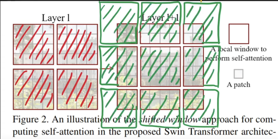
To explain furthermore on second layer, let’s look at the image below.

Shifted Windows in Swin Transformer

Let’s slowly wrap this, Swin Transformer, introduces a novel mechanism—Shifted Window Multi-head Self-Attention (SW-MSA)—to efficiently model long-range dependencies without incurring the high cost of global self-attention.

Why Shift Windows? The baseline attention mechanism, Window-based MSA (W-MSA), computes self-attention within non-overlapping windows. This is efficient, but it lacks cross-window communication.

To address this, shifted windows are applied in alternating Transformer blocks:

• Each window is shifted by a fixed size (e.g., half the window dimension).
• This causes adjacent windows to partially overlap.
• As a result, tokens from different regions can now interact, enhancing the model’s representational power.

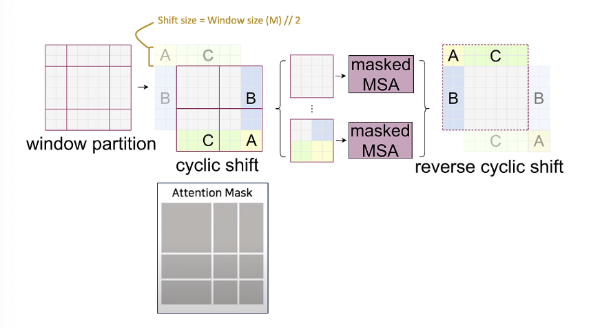
Cyclic Shift & Attention Masking

Shifting windows introduces new windows and disrupts alignment, potentially increasing computational complexity. Swin Transformer handles this elegantly using:

• Cyclic Shift:
  • Instead of moving data in memory, patches are cyclically shifted (like a ring buffer), preserving the GPU’s memory alignment and restoring the original number of windows. (ex: a left-side window is shifted down and right, aligning back to the initial layout.)
• Attention Masking:
  • After shifting, some patches may come from semantically unrelated areas.
  • Example: patches A, B, and C are visually close after the shift, but not contextually related.
  • A binary attention mask ensures that attention is only computed within valid, local regions.
  • After self-attention, the cyclic shift is reversed, restoring spatial structure.

Relative Positional Encoding

Unlike traditional Vision Transformers (ViT), which use absolute positional embeddings, Swin Transformer applies:

• No positional encoding at the input.
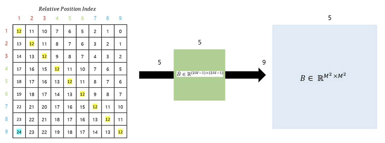
• Instead, relative position bias is learned and added during attention computation.
  • This bias represents the relative distance between tokens inside each window.
  • It enables the model to maintain spatial structure without global positional references.

• The details are shwon below

  $Attention(Q, K, V) = SoftMax(\frac{QK^T}{\sqrt{d}} + B)Vs$

In conclusion, as shown in the figure above, the Relative Position Bias is generated using $\hat{B}$. Ultimately, for the matrices $Q$, $K$, and $V$, where $M^2$ represents the number of Window Patches, and the relative positions along each axis range from $[-M+1, M-1]$, it can be seen that a smaller-sized Bias matrix $\hat{B}$ is parameterized, and the values of $B$ are derived from $\hat{B}$.

Resource

• Small Object Detection for Birds with Swin Transformer
• Swin Transformer: A Scalable Vision Transformer That just make sense
• Swin Transformer V1 Review
• Swin Transformer Paper Review
• Swin Transformer Paper Review
• Youtube - Swin Transformer Animated and Explained
• Youtube - Hierarchical Vision Transformer using Shifted Window

Attention Mechanism

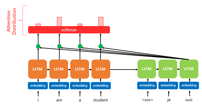
The basic idea of attention is that, at each time step during decoding, the decoder refers back to the entire input sentence encoded by the encoder. Instead of treating all parts of the input sentence equally, the model focuses more on the specific parts of the input that are most relevant to predicting the current output word.

Attention Function (HashMap Analogy)

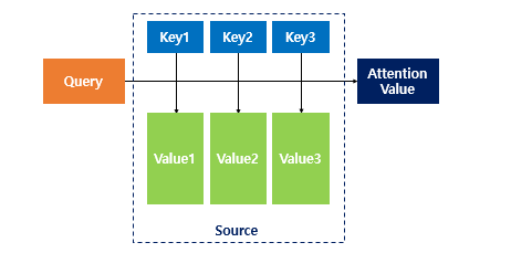
The attention function can be thought of similarly to a Python dictionary. However, its role is to compute the similarity between a given query and all keys, then map each key to a value weighted by this similarity. The output is essentially a weighted sum of these values, where the weights reflect the relevance (similarity) to the query.

• Q: Query — The hidden state of the decoder cell at time step 𝑡
• K: Keys — The hidden states of all encoder cells at every time step
• V: Values — The hidden states of all encoder cells at every time step

Attention Features

At each time step, the decoder refers back to all encoder hidden states, focusing more on the words that are most relevant. This approach helps address issues like vanishing gradients and the fixed-size output vector limitation of traditional RNNs.

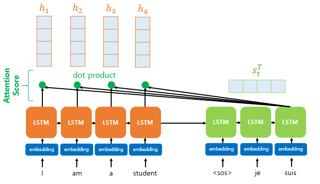
The attention mechanism computes similarity scores based on dot products. Specifically, to calculate the attention scores, the decoder’s hidden state at time step 𝑡, denoted as 𝑠𝑡, is multiplied by each encoder hidden state ℎ1, ℎ2, …,ℎ𝑁 For example, in the third decoding stage where the model predicts the next word after “je” and “suis,” it re-examines all encoder inputs to determine relevant information.

Formally, assuming the encoder and decoder hidden states share the same dimensionality, the attention scores 𝑒𝑡 can be calculated as: `et = [st⊤h1, st⊤h2, … ,st⊤hN] Here, 𝑒𝑡 is the vector of attention scores representing the relevance of each encoder hidden state to the current decoder state.

After computing the attention scores, we apply the softmax function to obtain the attention distribution, also known as the attention weights. By applying softmax to the attention scores 𝑒𝑡, we get a probability distribution 𝑎𝑡, where all values sum to 1. Each value in 𝑎𝑡 represents the weight (or importance) assigned to the corresponding encoder hidden state.

Formally: 𝑎𝑡 = softmax(𝑒𝑡) These attention weights determine how much each encoder hidden state should contribute to the current decoding step. In the diagram, the red rectangles represent the magnitude of attention weights applied to the encoder hidden states.

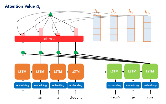
Once the attention weights 𝑎𝑡 are computed, we calculate the weighted sum of the encoder hidden states. This weighted sum is called the attention value, and it’s also commonly referred to as the context vector.

The higher the attention weight assigned to a particular hidden state, the more strongly it contributes to the final context vector—indicating a higher relevance to the current decoding step.

Formally, the context vector context 𝑡 (or attention value) is computed as: \[\text{context}_t = \sum_{i=1}^{N} a_i^t \cdot h_i\]

This vector summarizes the relevant parts of the input sequence, tailored for the current decoding time step 𝑡.

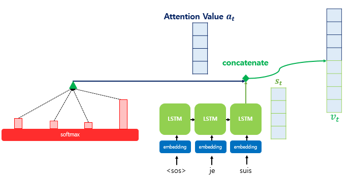
After computing the attention value (context vector), it is concatenated with the decoder’s hidden state at time step 𝑡, denoted as 𝑠𝑡.

This concatenated vector, often written as 𝑣𝑡 = [context𝑡;𝑠𝑡], combines both the information from the encoder (via attention) and the current state of the decoder. This merged vector 𝑣𝑡 is then used as input for predicting the output 𝑦𝑡, helping the model make more accurate predictions by leveraging both current decoding context and relevant encoder features.

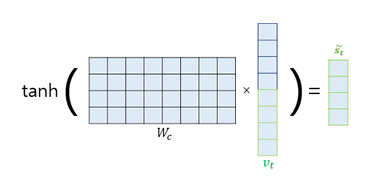
Computing ( \tilde{s}_t ), the Input to the Output Layer

Before sending ( v_t ) (the concatenation of the context vector and the decoder hidden state) directly to the output layer, it is passed through an additional neural layer for transformation.

Specifically, ( v_t ) is multiplied by a weight matrix and then passed through a hyperbolic tangent (tanh) activation function. This results in a new vector ( \tilde{s}_t ), which serves as the final input to the output layer: \[\tilde{s}_t = \tanh(W_o \cdot v_t)\]

This transformation allows the model to learn a richer representation before making the final prediction for the output word ( y_t ).

Different Attention & Score

RNN + Attention (seq2seq) Limitation

The Encoder-Decoder structure consists of two main components: the encoder, which compresses the input sequence into a fixed-length vector (often called the context vector), and the decoder, which generates the output sequence based on this vector.

However, this approach has several limitations:

• Information loss during compression into a single vector
• Lack of parallelism, since RNN-based encoders/decoders process sequences sequentially
• High computational complexity

To address these issues, the Transformer architecture was introduced.

Transformer

The Transformer replaces recurrence with attention mechanisms, specifically self-attention and cross-attention, to model dependencies in sequences. Just as CNNs use convolution to extract feature maps, attention computes similarity scores using dot products, followed by a weighted sum of values. This allows the model to focus on the most relevant parts of the input when processing each token.

Key features include:

• The ability to differentiate between individual tokens using attention weights
• The use of self-attention within both the input (encoder) and output (decoder) sequences
• Support for parallel computation, greatly improving training efficiency

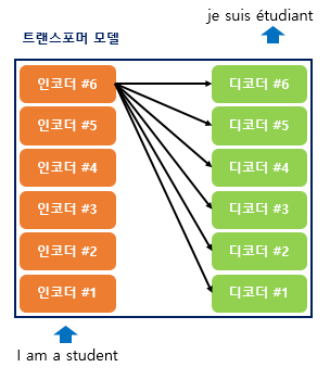
Although the Transformer does not use RNNs, it still follows the Encoder-Decoder architecture, where it takes an input sequence and generates an output sequence. The overall structure is similar to that of traditional RNN-based models.

However, there is a key difference: In RNNs, the model processes the sequence step by step over time — each unit corresponds to a specific time step 𝑡. In Transformers, the model processes the entire sequence in parallel. Instead of time steps, it consists of 𝑁 repeated encoder and decoder blocks, each operating on the entire sequence simultaneously. This structural shift allows Transformers to overcome the sequential bottleneck of RNNs and achieve much better performance in terms of parallelization and long-range dependency modeling.

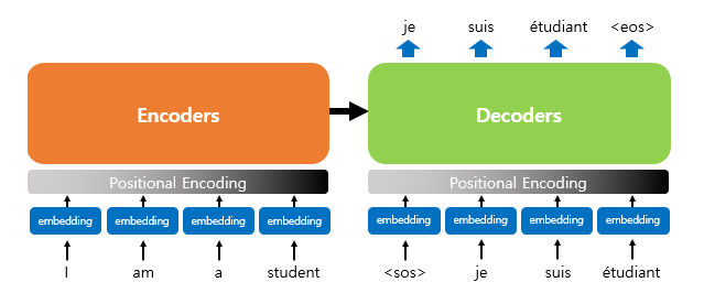
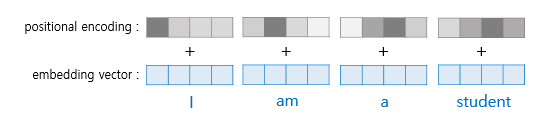
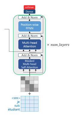
The end of the computation is as shown in the image below. The process continues from the input <sos> until <eos> is produced. Especially, since it is not divided by time steps like an RNN, positional encoding is necessary. In other words, a word’s one-hot encoding technique can be considered to be included.

Transformer Components

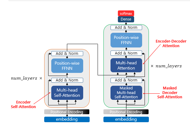
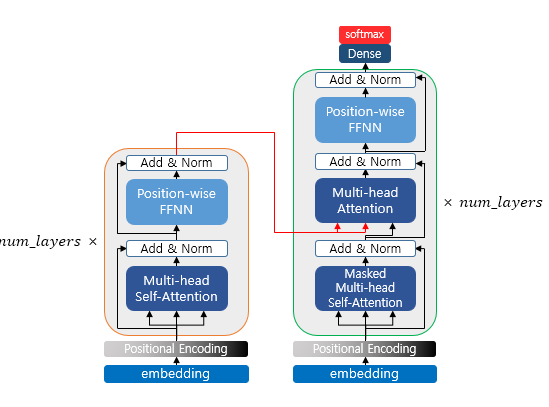
I will first define the following steps. The diagram below can be considered the overall architecture.

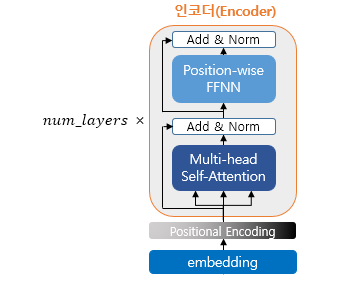
Encoder (self.attention)

The encoder is built using num_layers (6). Inside, there can be layers such as multi-head self-attention and position-wise FFNN.

In Sequence-to-Sequence models, the meaning of Q, K, and V was that Q represented the decoder hidden state at time step t.

However, in self-attention, Q, K, and V are the same. This means they represent the vectors of all words in the input sentence.

Note that instead of using the words themselves directly, their dimensionality is reduced. For example, if there are 4 words, each has a position vector, and these position vectors’ dimensions are reduced to form the dimensions of Q, K, and V.

After that, scaled dot-product attention is applied. Overall, this is performed as matrix operations (not just vector operations).

Multi-Head Attention

Among the parameters, there is a “number of heads,” which corresponds to parallel processing heads. Each head performs the following steps with Q and K: matrix multiplication → scaling → optional masking → softmax → matrix multiplication with V. Each head extracts different values, and by processing them in parallel, the values from each head are obtained.

Padding Mask

Here, the mask refers to the padding mask. Padding tokens have no actual meaning. Therefore, in the transformer, if a key corresponds to a padding token, similarity is not computed—in other words, it is excluded (which might be compared to a skip connection, but they are not the same). In this case, the padding mask has small values (close to zero) in the attention score.

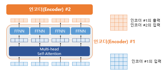
Position-wise FFNN

The point-wise FFNN can be considered a sublayer that both the encoder and decoder have. Therefore, it can be viewed as performing the computations shown in the diagram below.

Another notable aspect is the use of skip connections and layer normalization (similar to the residual blocks in ResNet).

Encoder to Decoder

That is, the encoded information is passed to the decoder. This is done by feeding the values into the multi-head attention. We will take a closer look at this part on the decoder side. If you want, I can help expand or clarify further!

Decoder (Self-Attention / Look-Ahead Mask)

Like the encoder, the decoder also receives a sequence of words as input. However, to prevent the model from looking at future words beyond the current time step, an optional mask is applied during training. This masking prevents the decoder from attending to subsequent words and is called the look-ahead mask. Similar to the encoder, self-attention is performed.

In summary, the decoder can only attend to itself and the previous words, but not to future words.

The second case is when the values received from the encoder and the decoder are used together. In this layer, it is not self-attention. This means the definitions of Q, K, and V are different.

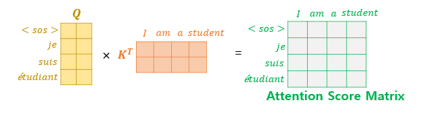
Q corresponds to the decoder matrix, while K and V correspond to the encoder matrix. Mapping this to the example above, it looks like the following.

After that, the output probabilities are generated, and during inference, the token with the highest probability is produced.

Dot Product of Query and Key Values

Resource

• WikiDocs - Deep Learning Approach for Natural Language Processing

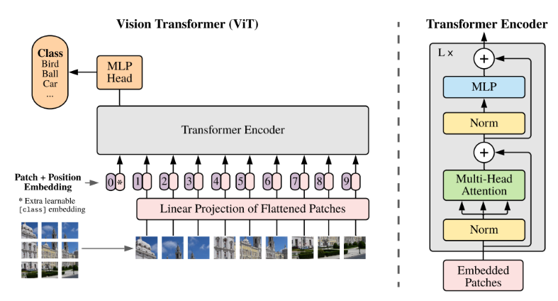
You might have seen this in previous posts. Essentially, a Transformer is a self-attention model that operates in the following way:
Normalization → Multi-head Attention → Normalization → MLP.

Let’s take a look at the overall architecture diagram below.

Input Data

Since it is a Vision Transformer, image data and the corresponding label data are used for training.

수식은 아래와 같다. \[x \in \mathbb{R}^{C \times H \times W}\]

Image Patch in Vision Transformers

In the context of Vision Transformers, an Image Patch refers to the process of dividing an input image into smaller, fixed-size segments called patches. These patches are typically of size $ p \times p $ pixels and are used as input to the Transformer model, effectively treating the image as a sequence of patches, similar to how words are treated in natural language processing.

For example:

• Given a 224 x 224 pixel image, if the patch size is set to 16 x 16 pixels, the image is divided into a grid of 14 x 14 patches (since $ 224 \div 16 = 14 $). Each patch is then flattened and processed as part of a sequence, which is fed into the Transformer architecture for vision tasks.

• This approach allows the Transformer to leverage its sequence-processing capabilities for vision tasks, treating the grid of patches as a sequence of “tokens” akin to words in text processing.

• Below is a direct translation of your input into English, formatted in Markdown, keeping the technical details and structure intact as requested.

CNNs and Vision Transformers: Image Patch Flattening CNNs have traditionally excelled in image processing through convolution operations. One of their drawbacks is the explosive increase in parameters, leading to issues like overfitting and gradient vanishing, which are addressed using regularization or dropout. In contrast, Transformers appear to rely on a specific exploitation method. In traditional Transformers, word embedding sequences are used as input. For vision tasks, this is adapted by inputting image patch sequences, enabling tasks like image label prediction. This represents a distinctly different architectural pattern. Flattening of Image Patches With patched images, a flattening process is applied to convert each patch into a vector of size $p^2 \times c$, where:

• Flatten Operation: The image is divided into patches, and each patch is flattened into a vector. Patch and Input Size: For an image of size $H \times W$ pixels divided into $N$ patches (where $N = \frac{HW}{p^2}$), each patch is processed.

• Flattened Vector: Each patch $z_p$ is represented as a vector in $\mathbb{R}^{N \times (p^2 \cdot c)}$, where:

• $p$: Size of one side of the patch.
• $c$: Number of color channels (e.g., 3 for RGB).
• $N = \frac{HW}{p^2}$: Total number of patches, derived from the image dimensions $H$ (height) and $W$ (width) divided by the patch area $ p^2 $.

Mathematical Formulation \(z_p \in \mathbb{R}^{N \times (p^2 \cdot c)} \quad \text{where} \quad N = \frac{HW}{p^2}\)

This reflects the process of converting image patches into a sequence of flattened vectors suitable for input into a Transformer model.

Patch Embeddings

After dividing the image into patches, embeddings are created from each patch. The split image patches undergo a linear transformation to initiate the encoding process. The resulting vectors are referred to as Patch Embedding Vectors, and they are characterized by a fixed length $ d $.

• Each patch of size $ n \times n $ is reshaped into a single column vector of size $n^2 \times 1$.
  • Example: A patch of $16 \times 16$ pixels is flattened into a $256 \times 1$ vector.

Linear Projection

Each patch, after flattening, concatenates all pixel channels. It then undergoes a linear projection to the desired input dimension. This might seem confusing, but the key idea is:

After flattening, each patch becomes a single column vector (e.g., $256 \times 1$). The linear projection aims to reduce or transform the dimensions, typically for compatibility with the model’s input requirements. Example: If a $256 \times 1$ flattened patch is input into a linear layer with 512 nodes, a linear computation (multiplication by weights plus addition of bias) transforms it into a $512 \times 1$ output vector.

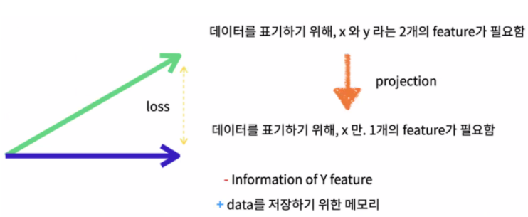
Projection of Two Features into One

By projecting two features into a single feature through linear projection, the process allows the use of only one feature. Ultimately, this maps pixel values into a format the model can understand. This involves transforming high-dimensional pixel data into a vector (or point), enabling a more concise representation that captures essential information.

Latent Vector Definition

The latent vector represents the encoded representation of the image patches after processing. It is defined as:

A sequence of $N$ patch embeddings, where each embedding is scaled by a factor $\alpha$. The resulting vector is denoted as $[\alpha^1 E_1, \alpha^2 E_2, \dots, \alpha^N E_N]$.

Mathematical Formulation \([\alpha^1 E_1, \alpha^2 E_2, \dots, \alpha^N E_N] \in \mathbb{R}^{N \times D}\) where:

$E \in \mathbb{R}^{(p^2 \cdot c) \times D}$: The embedding matrix, with $p^2 \cdot c$ representing the flattened patch size (where $p$ is the patch dimension and $c$ is the number of channels) and $D$ is the desired embedding dimension.

Through this process, all patches can be embedded into vectors. The result is an $ N \times D $ array, where:

• $N$: The number of patches.
• $D$: The embedding size for each patch.

This $N \times D$ array represents the embedded patch sequence ready for input into the Transformer model.

Appending a Class (Classification) Token

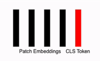
To effectively train the model, a vector called the CLS Token (Classification Token) is added to the patch embeddings. This vector: Acts as a learnable parameter within the neural network.

• Is randomly initialized.
• Is a single token added uniformly to all data instances.

After this step, the total number of embeddings becomes $n + 1$ (where $n$ is the number of patch embeddings plus the CLS token). Combined with the embedding size $D$, this results in a $(n+1) \times D$ array, which serves as the representation vector for further processing.

Initial Embedding with CLS Token

The initial embedding $ z_0 $ is formed by appending the CLS Token to the patch embeddings. It is defined as:

Mathematical Formulation \(z_0 = [\alpha_{cls}, \alpha^1_p E_1, \alpha^2_p E_2, \dots, \alpha^N_p E_N] \in \mathbb{R}^{(N+1) \times D}\)

• $\alpha_{cls} $: The CLS Token, a learnable vector.
• $\alpha^1_p E_1, \alpha^2_p E_2, \dots, \alpha^N_p E_N$: The scaled embeddings of $N$ patches.
• $(N+1) \times D$: The resulting dimension, where $N$ is the number of patches and $D$ is the embedding size.

This $z_0$ serves as the input representation vector for the Transformer model.

Adding Positional Embedding Vectors

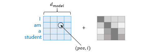
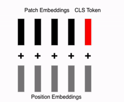
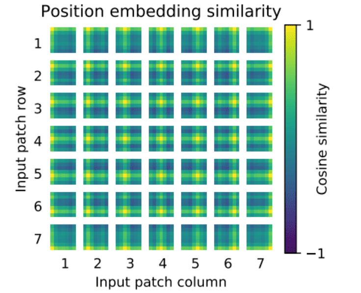
In the original Transformer, positional information for words was added to create 2D data. For images, where “which position?” becomes relevant, a process is added to encode positional information for each patch, reflecting its spatial location. This positional encoding is directly added to each embedding vector, including the CLS Token.

Process

• Patch Embeddings: Represent the content of each patch.
• Positional Embeddings: Encode the spatial order or position of each patch.
• Combination: The positional embeddings are added to the patch embeddings and the CLS token to form the final input.

The Equations are following:

$z_0 = [\alpha_{cls}, \alpha^1p E_1, \alpha^2_p E_2, \dots, \alpha^N_p E_N] + E{pos} \in \mathbb{R}^{(N+1) \times D}$

where:

• $E_{pos} \in \mathbb{R}^{(N+1) \times D}$: The positional embedding matrix, with the same shape as the patch and CLS token sequence. This $z_0$ represents the final input to the Transformer, incorporating both the content (via patch embeddings and CLS token) and positional information.

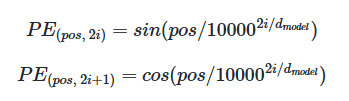
Similar to the previous discussion, the positional encoding method used here involves sin and cos functions, as seen in prior posts. This approach encodes the positional information of each patch, allowing the model to understand the spatial arrangement of the image patches.

The positional encoding $ PE(pos, 2i) $ and $ PE(pos, 2i+1) $ are defined using sine and cosine functions to encode the position of each patch. The formulas are: Mathematical Formulation \(PE(pos, 2i) = \sin\left(\frac{pos}{10000^{2i/d_{model}}}\right)\) \(PE(pos, 2i+1) = \cos\left(\frac{pos}{10000^{2i/d_{model}}}\right)\)

• $pos$: The position of the patch.
• $i$: The dimension index.
• $d_{model}$: The dimensionality of the model.

Encoder

Encoder Input

After the previous steps, you now have an array of size $(n + 1) \times d$, where $n$ is the number of patches and $ d $ is the embedding dimension. The next step is to apply self-attention, which allows the model to weigh the importance of different patches (including the CLS token) in relation to each other.

Multi-Head Self Attention

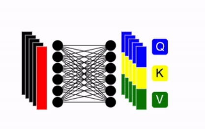
Create QKV (Query, Key Value)

The embedding vector generated from the previous steps is linearly transformed into multiple large vectors, which are subdivided into three components: Q (Query), K (Key), and V (Value). These vectors are derived from the $(n + 1) \times d$ array, where $n + 1$ represents the number of patches plus the CLS token, and each component retains the same $n + 1$ length.

The equations are following: \[q = z \cdot w_q,\quad k = z \cdot w_k,\quad v = z \cdot w_v \quad \text{where} \quad w_q, w_k, w_v \in \mathbb{R}^{D \times D_h}\]

• usually, $D_h$ set to $D/k$, (k is the number of attention heads — enabling parallel processing.)

Self.Attention

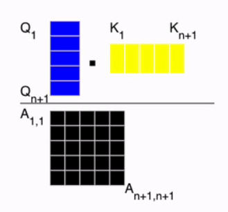
Now, we need to compute the attention score. As shown in the image below, the similarity is calculated by taking the dot product between the query and the key. Then, softmax is applied so that the sum of each row in matrix ( A ) becomes 1.

The equations are following: \[SA(z) = A \cdot v \in \mathbb{R}^{N \times D_h}, \quad \text{where} \quad A = \text{softmax} \left( \frac{q \cdot k^T}{\sqrt{D_h}} \right) \in \mathbb{R}^{N \times N}\]

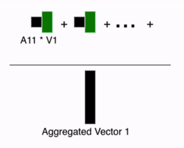
After that, a weighted sum is computed over ( v ) using the attention weights.

Here’s the process: to obtain the aggregated contextual information for each element, we perform the computation using the first row of the attention matrix. At this point, we use the weights applied to ( V ) to generate the aggregated vector for the first image embedding. This operation is then applied to all patches.

Multi-Head Attention

The above process is ultimately repeated multiple times. \[MSA(z) = [SA_1(z); SA_2(z); \cdots; SA_k(z)] U_{\text{msa}} \quad \text{where} \quad U_{\text{msa}} \in \mathbb{R}^{(k \cdot D_h) \times D}\]

MLP (Additional Details)

• Pretraining: Uses one hidden layer.
• Finetuning: Uses a single linear layer.
• In total, two linear layers are used, along with the GELU (Gaussian Error Linear Unit) activation function.

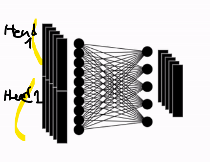
Last Attention Layer Setup

After stacking multiple attention heads, the result is mapped to a vector of dimension ( D ), which matches the patch embedding size.

Attention Layer Result

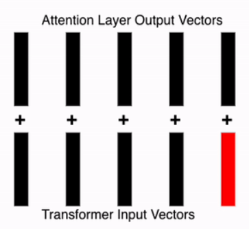
Residual Connection

Simply adds the input from the previous layer to the current layer.

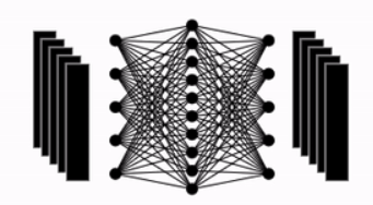
Feed Forward Network

The output from the previous steps is passed into a feed-forward network.

Repeating Process

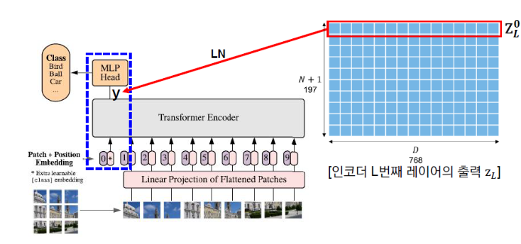
Repeat the above process L times. As shown in the second figure below, after L repetitions, the final classification is performed by passing the first vector y of the Encoder’s final output through an MLP Head consisting of a single hidden layer (dimension D × C).

Transformer Layer Processing

The output $z_l$ at layer $l$ is computed by applying a Multi-Layer Perceptron (MLP) and Layer Normalization (LN) to the input $z_l’$, combined with the residual connection $z_l$. The process is defined as:

Mathematical Formulation \(z_l = MLP(LN(z_l')) + z_l \quad \text{for} \quad l = 1, 2, \dots, L\) where: \(LN(z_l') = \gamma \frac{z_l' - \mu_i}{\sqrt{\sigma_i^2 + \epsilon}} + \beta\)

• $LN$: Layer Normalization.
• $MLP$: Multi-Layer Perceptron.
• $\gamma, \beta$: Learnable scaling and shift parameters.
• $\mu_i$: Mean of the input.
• $\sigma_i^2$: Variance of the input.
• $\epsilon$: Small constant for numerical stability.

This iterative process refines the embeddings across $L$ layers.

Identifying Classification Token Output and Predicting Classification Probabilities

The final step involves examining the output of the CLS Token (Classification Token). This vector serves as the last step in the Vision Transformer. In the final stage, it is passed through a Fully Connected Layer to compute Classification Probabilities, enabling the prediction of the image class.

Inductive Bias

• The term Inductive Bias frequently appears in this context. For CNNs, the use of Convolution Operations, which are specific to images, introduces an inductive bias. This bias includes:

• Locality: Focusing on local regions of the image.
• Two-Dimensional Neighborhood Structure: Capturing spatial relationships in a 2D grid.
• Translation Equivariance: Ensuring the model responds consistently to translated inputs.

In contrast, Vision Transformers (ViTs) rely on MLP Layers to implicitly address Locality and Translation Equivariance. ViTs learn these properties through the Input Image Patches and refine them via Positional Embeddings (e.g., through fine-tuning).

Resource

Transformers for Image Recognition at Scale