3D Gaussian Splatting Experiments

10 Feb 2026 in Study on Computer Graphics, Deep learning

Motivation

In the previous post, we looked at the history of Gaussian Splatting. Now, let’s look at some experiments with 3D Gaussian Splatting and validation of the results. Also, I want to learn this as kinda of like top-down approach. So, I will start with running the 3DGS pipeline on a custom dataset and then analyze the results. The goal is to understand how the pipeline works end-to-end and to validate that it produces reasonable results on a real-world scene.

Objective

It was to run the 3DGS implementation en-to-end on a custom dataset. (self-capmtured indoor scene) for the first time and validate the results.

Experience the full pipeline: COLMAP SfM → 3DGS training → point cloud output → viewer visualization
Verify that training converges and produces visually reasonable results on a custom scene
Obtain baseline quantitative metrics (PSNR / SSIM / LPIPS) for future comparison

First Run Gaussian Splatting.

The meta for first time running the 3DGS pipeline on playroom dataset. (225 Images). My GPU was NVIDIA GeFORCE RTX 2070 Super (8GB VRAM) and the training took about 2 days to complete. The viewer were used to visualize the output point cloud.

The config was as follows:

Namespace(
  data_device='cuda',
  eval=False,            # ← BUG: no train/test split → metrics are NaN
  images='images',
  resolution=-1,         # original resolution
  sh_degree=3,           # Spherical Harmonics degree
  source_path='C:\\Users\\skcjf\\project\\gaussian-splatting\\data\\my_scene\\playroom',
  model_path='./output/858ba1ea-e',
  train_test_exp=False,
  white_background=False
)

Results

Training time: ~2 days (RTX 2070 Super)
Iterations: 30,000 (checkpoints at 7,000 and 30,000)
Output: gaussian-splatting\output\858ba1ea-e\point_cloud\iteration_30000

Then I did not get the results that I expected because I did not add –eval flag to the config, so I got NaN for all the metrics. But the point cloud output looked reasonable and the viewer visualization showed a decent reconstruction of the scene. The PSNR, SSIM, and LPIPS metrics were not computed due to the missing evaluation flag, so I will need to rerun with –eval to get those quantitative results.

alt text

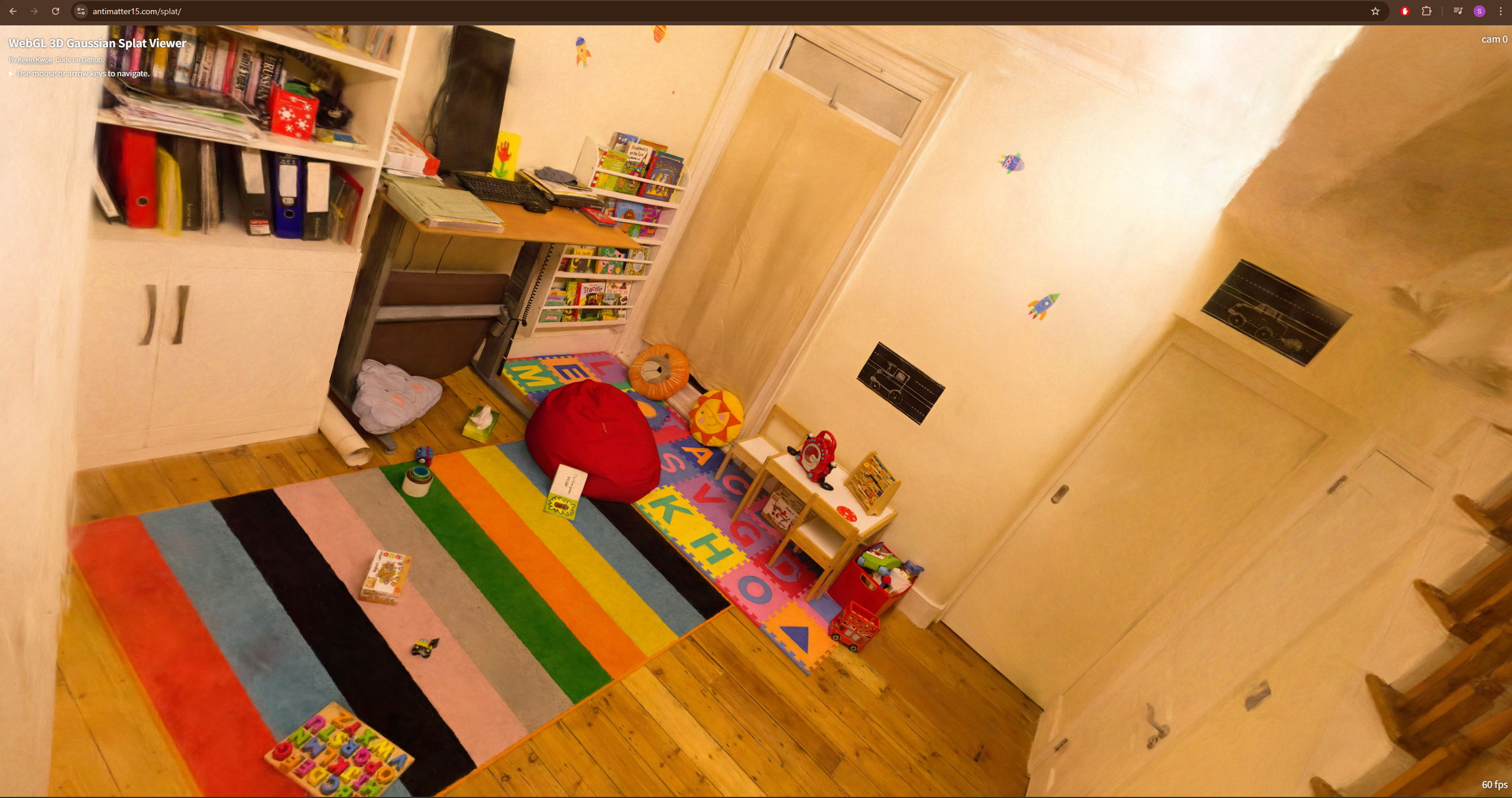
Iteration Comparison in Point Cloud Output:

Iteration	7K	30K

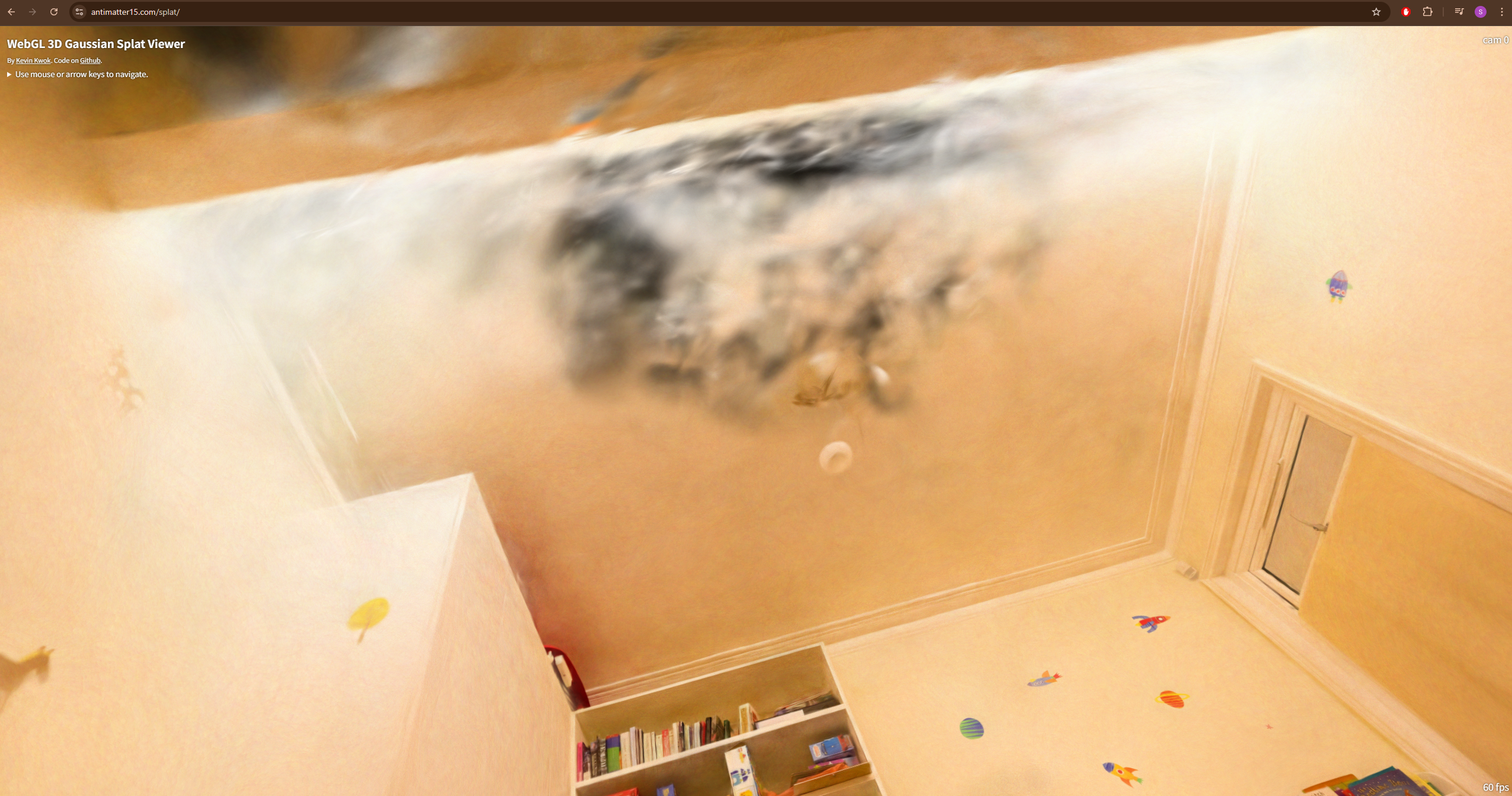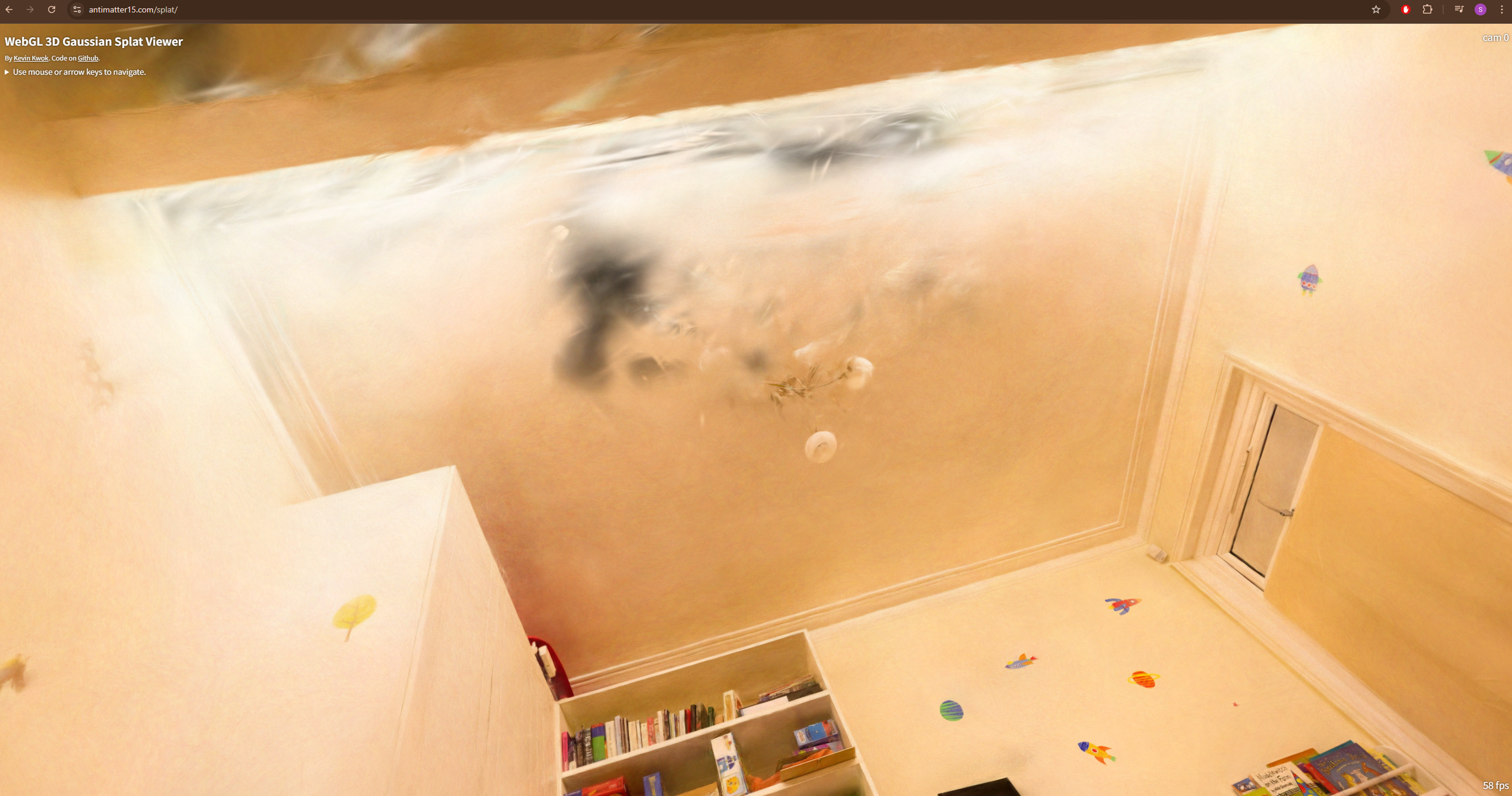Front-facing view (looking into the room): 7k and 30k are nearly identical
Looking up at the ceiling: visible holes/gaps → likely insufficient training views from upward angles, or densification did not cover that region adequately

Problem Encountered:

Output folder names are random hashes (e.g. 858ba1ea-e), so locating the actual results was initially confusing
No build errors; used a separate Python virtual environment
Training took ~2 days on RTX 2070 Super, which saturated the GPU entirely (couldn’t even run YouTube simultaneously)
4 total attempts, 3 failed/aborted before the successful run

Second Run with Evaluation

Objective

Run 3DGS on a standard benchmark dataset with --eval enabled to obtain real quantitative metrics (PSNR/SSIM/LPIPS) for the first time. This fixes the [[3DGS First Run]] problem where eval=False produced NaN metrics.

Validate that the 3DGS pipeline produces results consistent with the original paper
Establish a quantitative baseline for future experiments (hyperparameter tuning, ablation)
Learn the full evaluation pipeline: train → render → metrics

I choose to use Google Colab for this run to leverage a more powerful GPU (A100 40GB with High RAN) and faster training times. Then, I ran multiple data (tandt_db / Mip-NeRF 360 dataset) as well to validate the results from paper.

The config was as follows:

Namespace(
  sh_degree=3,
  source_path='/content/gaussian-splatting/data/tandt/train',
  model_path='/content/drive/MyDrive/3dgs_output/train',  # NOTE: mislabeled — actual scene is "train"
  images='images',
  resolution=-1,         # original resolution
  white_background=False,
  train_test_exp=False,
  data_device='cuda',
  eval=True              # FIXED from First Run — train/test split enabled
)

Results

Metric	Value
PSNR	22.12
SSIM	0.822
LPIPS	0.196
Gaussians	1,095,714
Iterations	30,000 (checkpoints at 7,000 / 30,000)
GPU	A100 40GB (Google Colab)

These were the metrics using for the dataset: tandt_db(train). The PSNR and SSIM values are consistent with the original 3DGS paper, which reported PSNR around 22-23 and SSIM around 0.8 for similar scenes. The LPIPS value of 0.196 also indicates a reasonably good perceptual quality compared to the ground truth images. The number of Gaussians (1,095,714) is also in line with expectations for a scene of this complexity.

Problems Encountered

Mip-NeRF 360 dataset URL (storage.googleapis.com) returned 404 — dead link
Initial !unzip extracted to wrong path → Could not recognize scene type! error. Fixed by ensuring sparse/0/ was in the correct location.

What I Learned

--eval is mandatory for quantitative evaluation — without it, no train/test split occurs
3DGS with default config on standard benchmarks reproduces paper results — the pipeline works
A100 vs RTX 2070 Super is a massive speed difference — Colab is the practical choice for experimentation
Dataset URL availability is not guaranteed — always have backup sources

Third Run with Mip-NeRF 360 Dataset

Objective

Experimentally verify the impact of 3 key 3DGS hyperparameters on the Mip-NeRF 360 dataset:

sh_degree: Spherical Harmonics degree (controls angular detail) for Kitchen Scene

The goal is to understand how these hyperparameters affect the final rendered quality (PSNR/SSIM/LPIPS) and visual appearance of the output point cloud. I will run multiple experiments varying one hyperparameter at a time while keeping others fixed, and then analyze the results.

Platform:

Google Colab with A100 High RAM for all experiments to ensure consistent training times and results.

Hyperparameter 1: Spherical Harmonics Degree (`sh_degree`)

Kitchen scene contains many reflective surfaces — stainless steel appliances, faucets, tiles
Higher SH degree enables more detailed view-dependent color changes (specular, highlights) as camera angle changes
Degree 0 = flat color (diffuse only), Degree 3 = highlights and reflections supported

Parameters:

# sh0
python train.py -s data/mipnerf360/kitchen --eval --sh_degree 0 -m .../kitchen/sh0
# sh1
python train.py -s data/mipnerf360/kitchen --eval --sh_degree 1 -m .../kitchen/sh1
# sh2
python train.py -s data/mipnerf360/kitchen --eval --sh_degree 2 -m .../kitchen/sh2
# sh3 (default)
python train.py -s data/mipnerf360/kitchen --eval --sh_degree 3 -m .../kitchen/sh3

Results

| Degree | SH Coefficients | SSIM | PSNR | LPIPS | Iterations | | —— | ————— | ——— | ———- | ——— | ———- | | 0 | 1 | 0.9244097 | 30.6005344 | 0.1243820 | 7k | | 1 | 4 | 0.9281715 | 31.0590820 | 0.1205885 | 7k | | 2 | 9 | 0.9311565 | 31.2686272 | 0.1176810 | 30k | | 3 | 16 | 0.9326434 | 31.5447502 | 0.1158840 | 7k |

Note: sh0, sh1, sh3 trained at 7k iterations, sh2 at 30k → metrics for sh2 may be overestimated. Re-run with unified iteration count for fair comparison.

Image Index	Description	Image
18	SH degree 0 ~ 3 with ground truth Comparison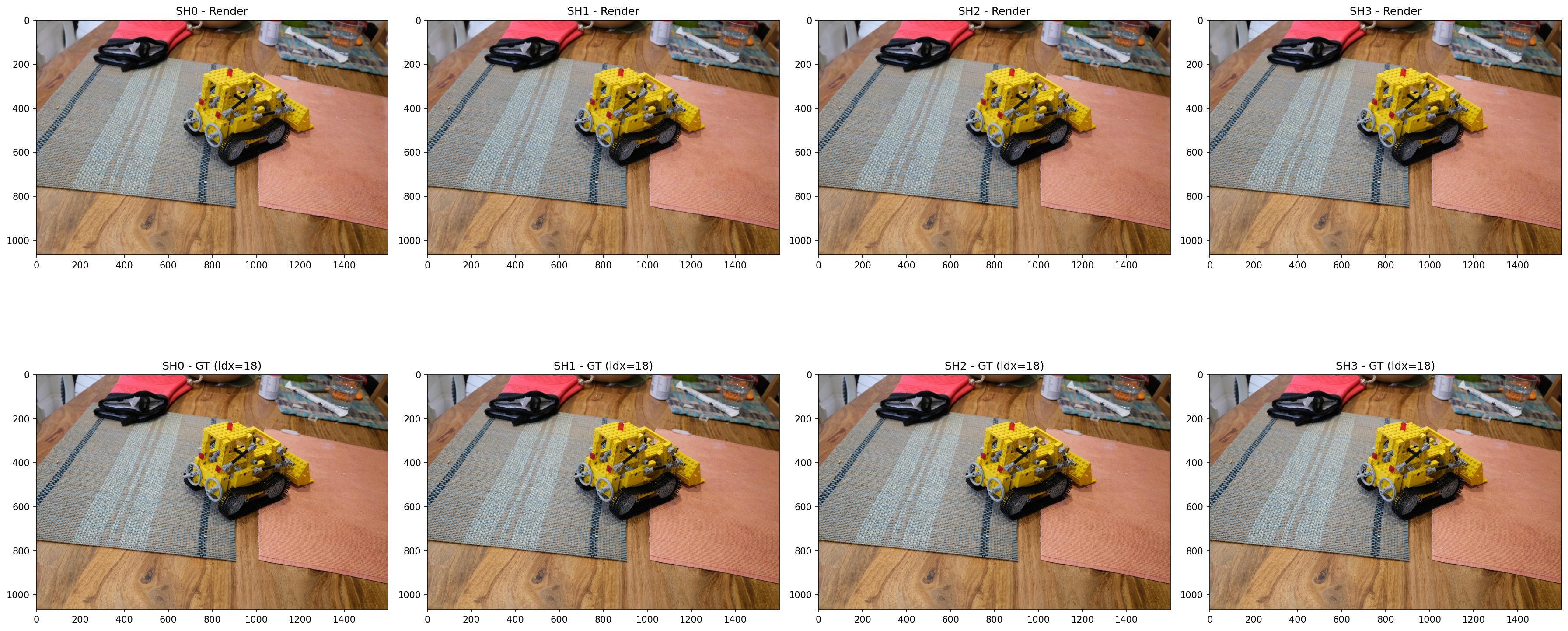
20	SH degree 0 ~ 3 with ground truth Comparison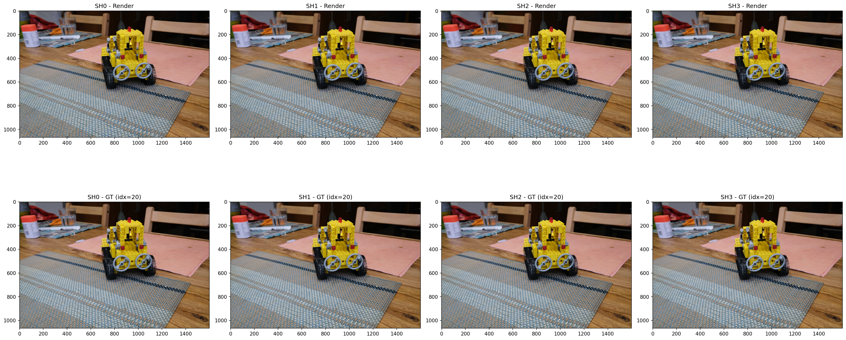
23	SH degree 0 ~ 3 with ground truth Comparison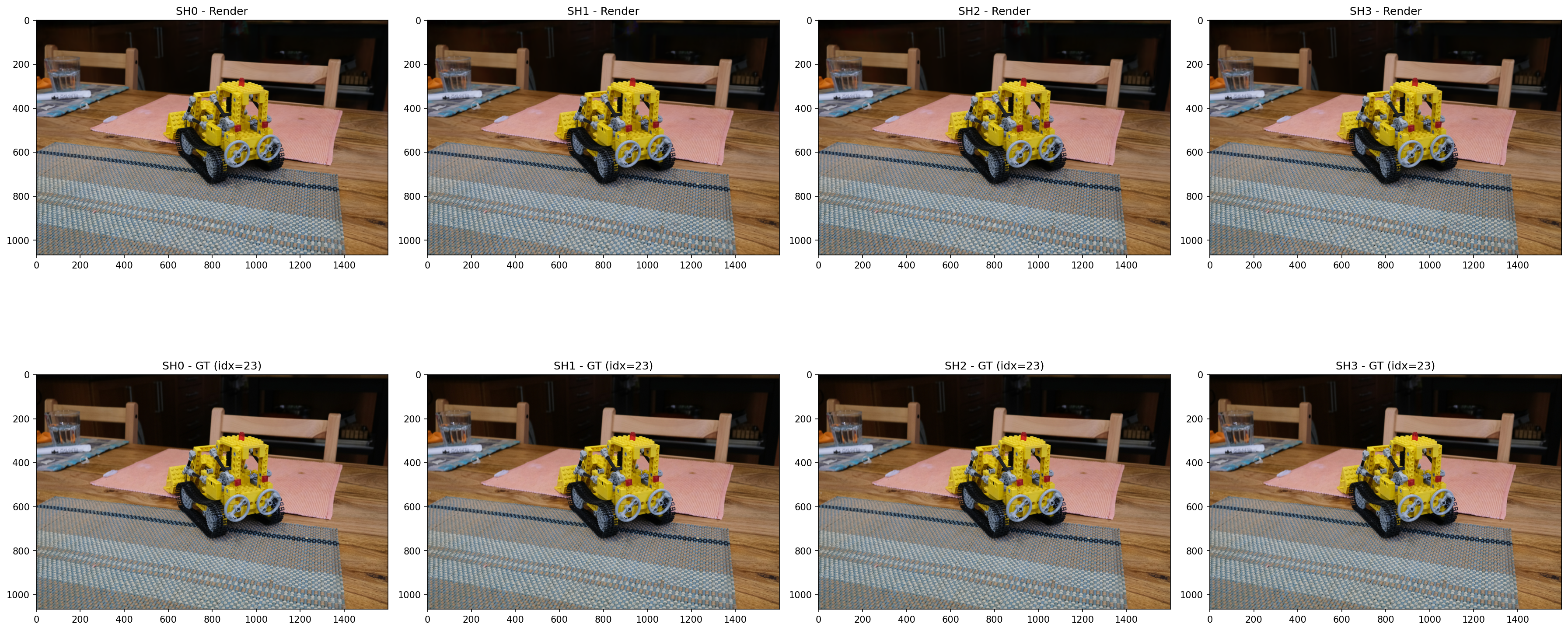

Hyperparameter 2: Densify Grad Threshold (`densification`)

Controls when Gaussians are split/cloned during training based on the gradient magnitude
Lower threshold → more aggressive densification → more Gaussians generated → better representation of thin structures (e.g. bicycle spokes, tree branches)
Higher threshold → fewer Gaussians → faster training but worse representation of fine details
Bicycle scene contains many thin structures (spokes, leaves, handlebars) that may benefit from aggressive densification and require 1–2 pixel level detail reconstruction

Parameters:

# Low (more Gaussians, detail ↑, VRAM ↑)
python train.py -s data/mipnerf360/bicycle --eval --densify_grad_threshold 0.0001 -m .../bicycle/dense_low

# Medium (default)
python train.py -s data/mipnerf360/bicycle --eval --densify_grad_threshold 0.0002 -m .../bicycle/dense_med

# High (fewer Gaussians, faster, detail ↓)
python train.py -s data/mipnerf360/bicycle --eval --densify_grad_threshold 0.0005 -m .../bicycle/dense_high

Results (30k iterations)

Threshold	Config	SSIM	PSNR	LPIPS
0.0001	Low	0.7719774	25.3083401	0.1857106
0.0002	Medium (Base)	0.7473353	25.1360970	0.2421628
0.0005	High	0.6516691	24.1706982	0.3792148

Image Index	Description	Image
0	Densification Threshold Comparison (0.0001, 0.0002, 0.0005) with GT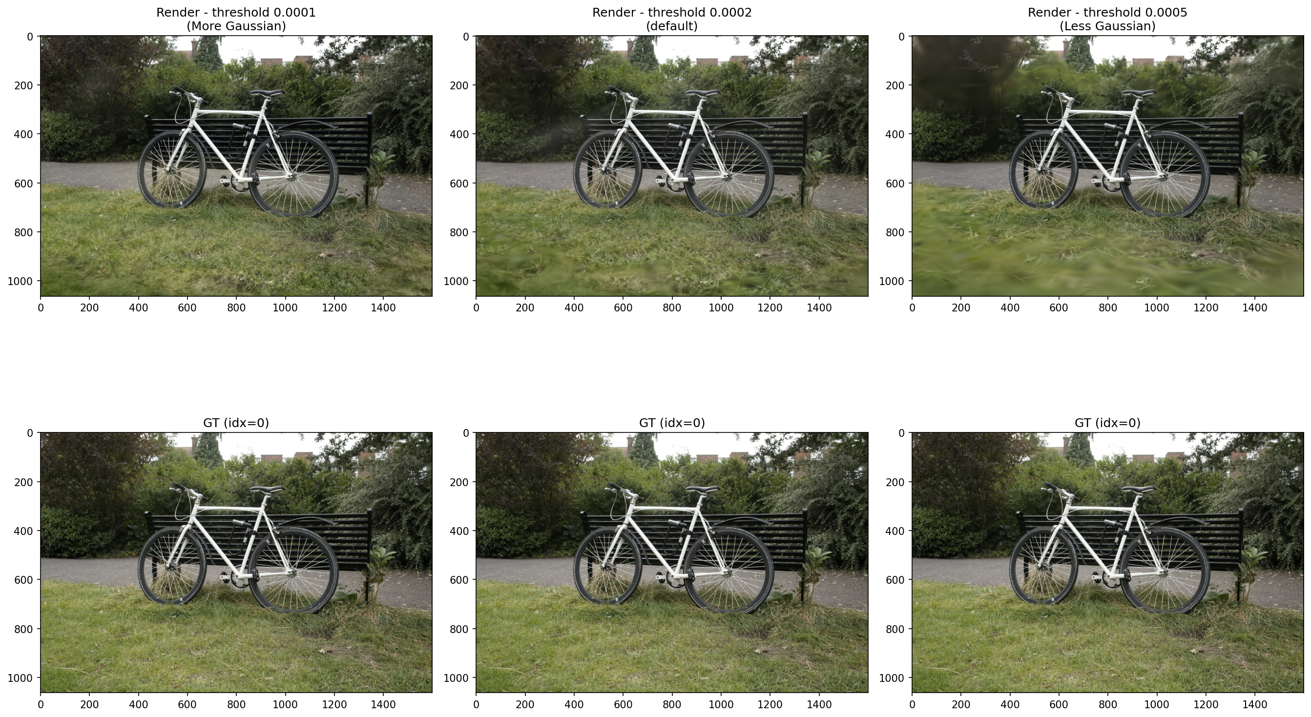
1	Densification Threshold Comparison (0.0001, 0.0002, 0.0005) with GT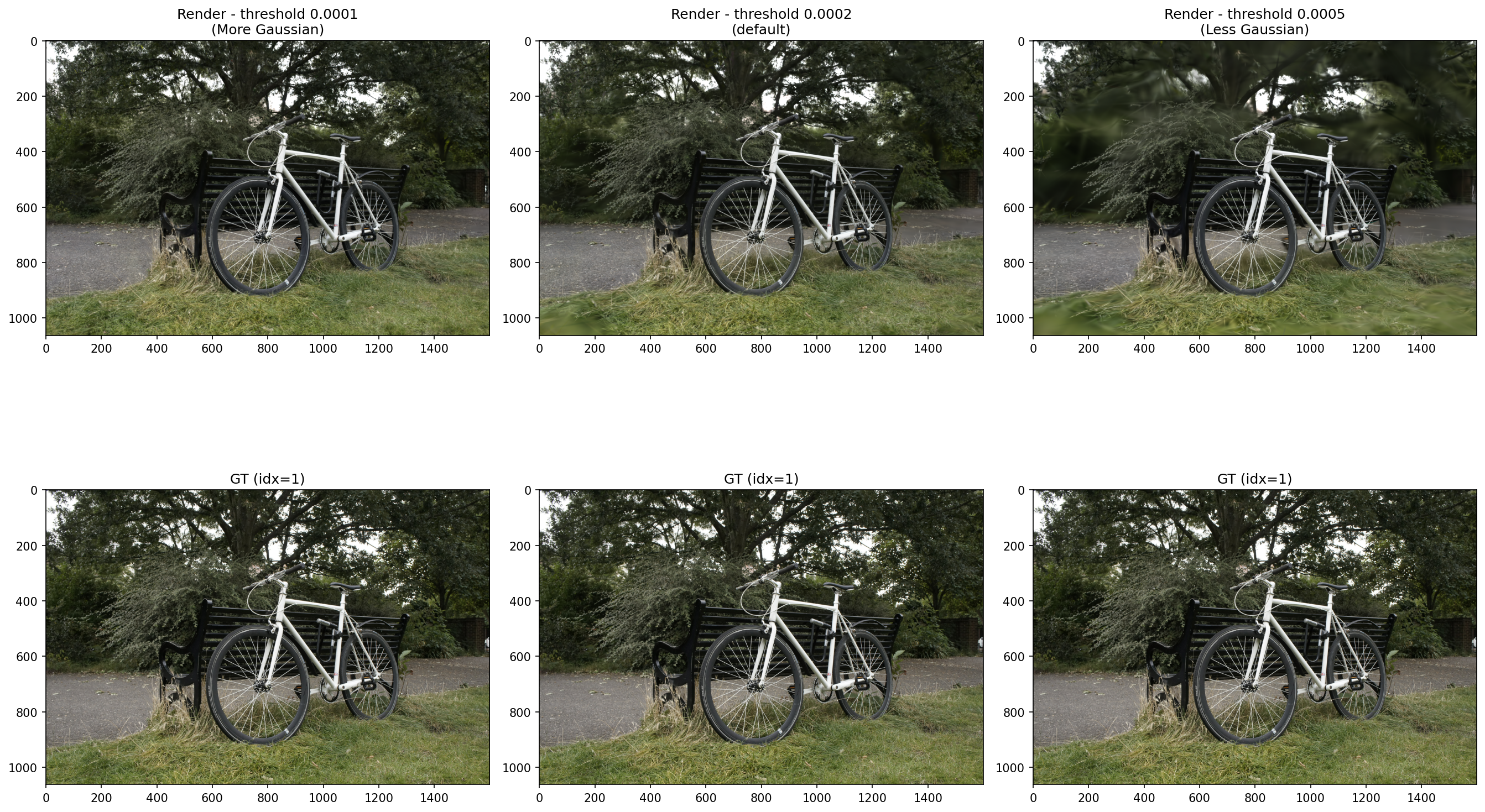
2	Densification Threshold Comparison (0.0001, 0.0002, 0.0005) with GT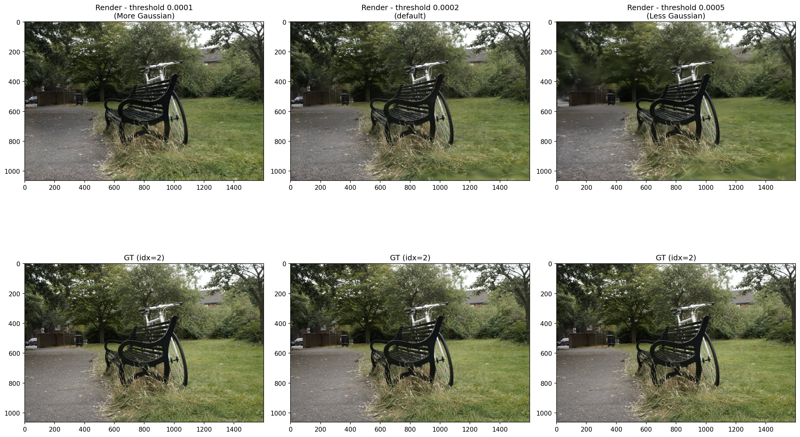

Observations

SH degree 0: Reflective surfaces appear as flat, uniform color. No highlights
SH degree 3: Highlights on pots and faucets shift as the camera angle changes
Higher degree increases view-dependent effects but also increases VRAM usage and training time
Diminishing returns: 0→1 gives the largest PSNR gain (+0.46), subsequent steps are smaller
Observations
Lower threshold (more Gaussians) = higher PSNR/SSIM and lower LPIPS → better across all metrics
LPIPS degrades more than 2x from Low → High (0.186 → 0.379) → thin structures deteriorate sharply
However, more Gaussians = higher VRAM usage → memory constraints must be considered in practic

Hyperparameter 3: Number of Training Iterations (`iterations`)

Objective

Does longer training improve quality? like NeRF?
At what point does the model converge?

Parameters:

# 7k
python train.py -s data/mipnerf360/bonsai --eval --iterations 7000 --densify_until_iter 5000 -m .../bonsai/iter7k

# 30k (default)
python train.py -s data/mipnerf360/bonsai --eval --iterations 30000 -m .../bonsai/iter30k

# 50k
python train.py -s data/mipnerf360/bonsai --eval --iterations 50000 --densify_until_iter 25000 --test_iterations 7000 30000 50000 --save_iterations 7000 30000 50000 -m .../bonsai/iter50k

Results

Iterations	SSIM	PSNR	LPIPS	PSNR Gain
7k	0.9323797	30.5002346	0.2045038	-
30k	0.9468836	32.3352585	0.1800254	+1.84
50k	0.9468449	32.6032143	0.1798774	+0.26

Image Index	Description	Image
5	Iteration Comparison (7k, 30k, 50k) with GT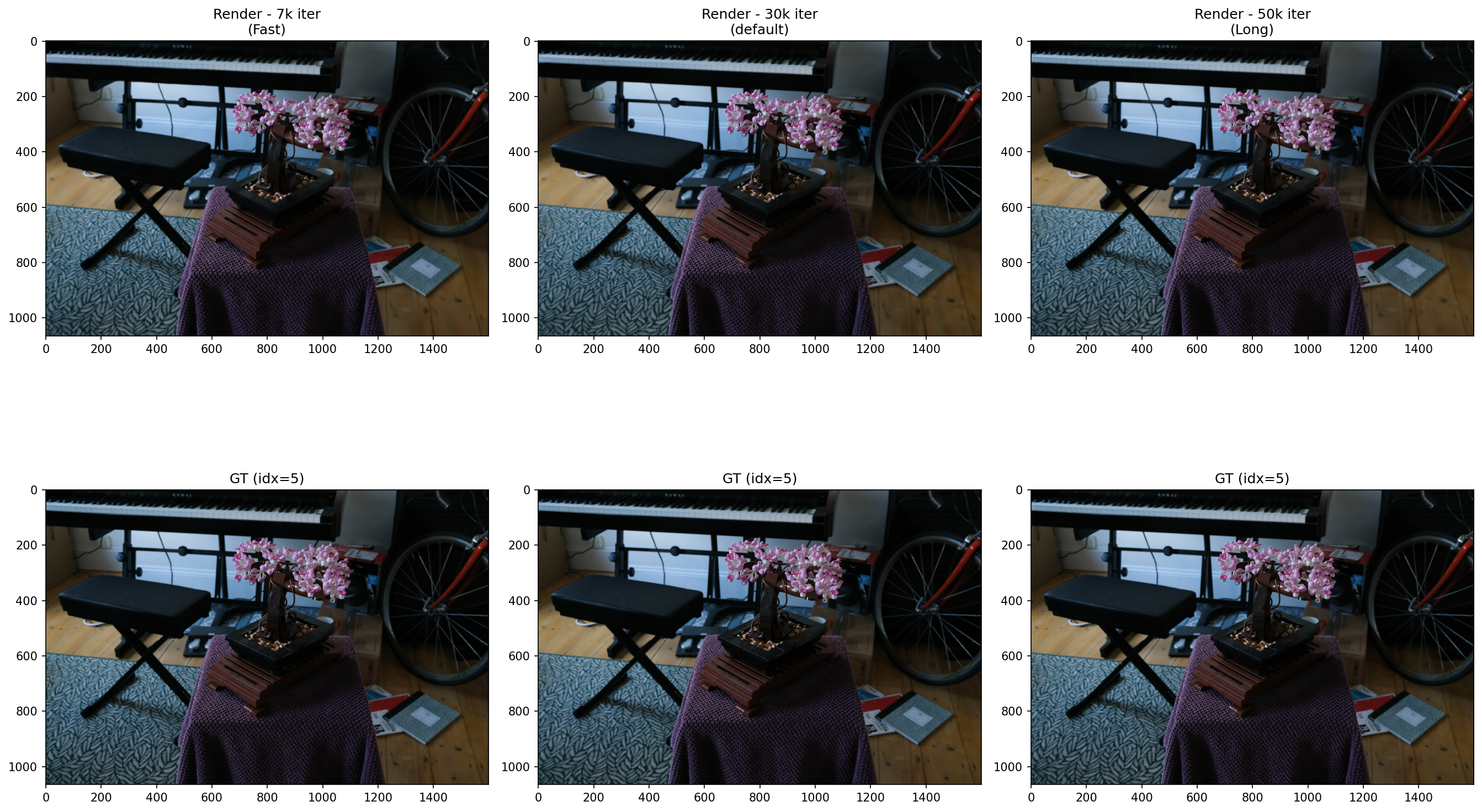
10	Iteration Comparison (7k, 30k, 50k) with GT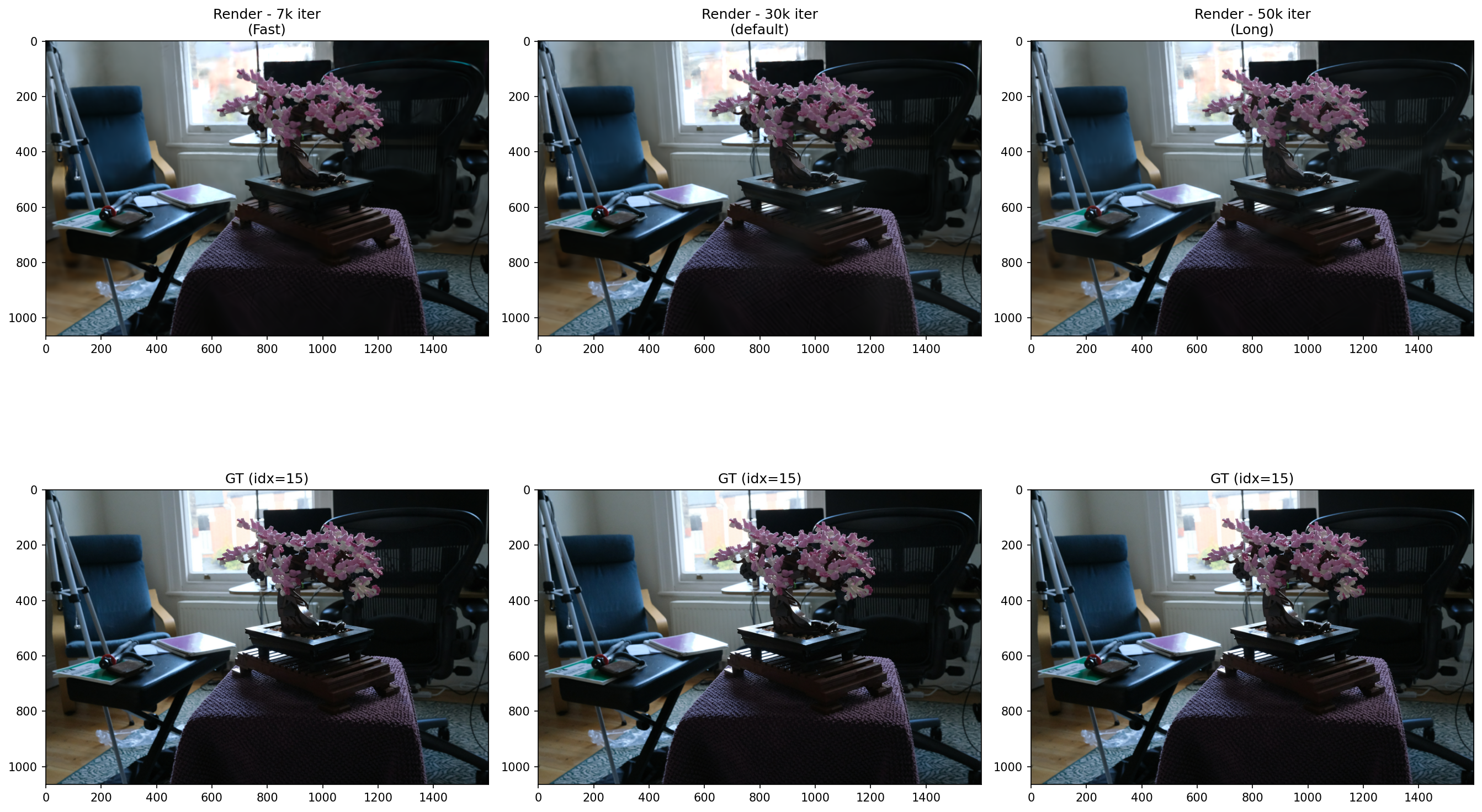
15	Iteration Comparison (7k, 30k, 50k) with GT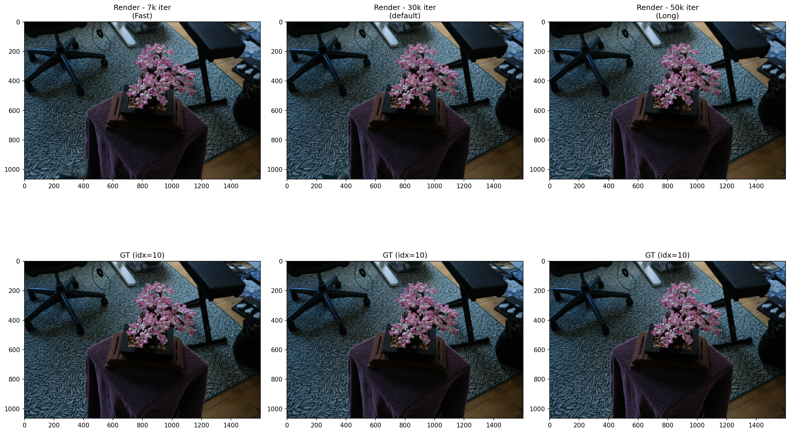

Observations

7k → 30k: PSNR +1.84 improvement. Leaf and stem sharpness clearly improved
30k → 50k: PSNR +0.26, SSIM nearly identical (0.9468) → convergence confirmed
Conclusion: 3DGS converges at ~30k iterations. Training beyond 50k yields diminishing returns

Summary

Experiment	Key Variable	Conclusion
Spherical Harmonics Degree	View-dependent color	Higher degree improves PSNR/SSIM and reduces LPIPS. Re-run with unified iterations for fair comparison
Densify Threshold	Gaussian count / thin structures	Lower threshold = better quality. VRAM trade-off exists
Iterations	Training time vs quality	Converges at 30k. Beyond 50k is inefficient

Resource

Repo History: https://github.com/sjang1594/3dgs-experiments/tree/main/experiments

3D Gaussian Splatting Experiments

Motivation

Objective

First Run Gaussian Splatting.

Results

Problem Encountered:

Second Run with Evaluation

Objective

Results

Problems Encountered

What I Learned

Third Run with Mip-NeRF 360 Dataset

Objective

Platform:

Hyperparameter 1: Spherical Harmonics Degree (`sh_degree`)

Results

Hyperparameter 2: Densify Grad Threshold (`densification`)

Results (30k iterations)

Observations

Observations

Hyperparameter 3: Number of Training Iterations (`iterations`)

Objective

Results

Observations

Summary

Resource

SJ.Home

Error

Motivation

Objective

First Run Gaussian Splatting.

Results

Problem Encountered:

Second Run with Evaluation

Objective

Results

Problems Encountered

What I Learned

Third Run with Mip-NeRF 360 Dataset

Objective

Platform:

Hyperparameter 1: Spherical Harmonics Degree (sh_degree)

Results

Hyperparameter 2: Densify Grad Threshold (densification)

Results (30k iterations)

Observations

Observations

Hyperparameter 3: Number of Training Iterations (iterations)

Objective

Results

Observations

Summary

Resource

Templates (for web app):

Error

Hyperparameter 1: Spherical Harmonics Degree (`sh_degree`)

Hyperparameter 2: Densify Grad Threshold (`densification`)

Hyperparameter 3: Number of Training Iterations (`iterations`)